STAB22H3 Lecture Notes - Lecture 11: Scatter Plot


38
STAB22H3 Full Course Notes
Verified Note
38 documents
Document Summary
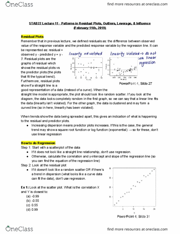
Coefficient of determination (r2) p211: the square of the correlation (r2) is the fraction of the variation in the values of y that is explained by the least-squares regression of y on x. In the above example r2=0. 979=97. 9%, i. e. 97. 9% of the variation is sales is explained by the regression of sales on ad. cost. Residual plots p208: residual plots help us assess the model assumptions. Doing regression: start with a scatterplot, otherwise, can calculate correlation and also intercept and slope of regression. If it does not look like a straight line relationship, stop line: check whether regression is ok by looking at plot of residuals against anything relevant. If not ok, do not use r egression: aim: want regression for which line is ok, confirmed by looking at scatterplot and residual plot(s). Patterns on residual plots pg. 237: example: population (in millions) in a country for 2000 2005 (recorded as.