STA 101 Chapter Unit 6: STATS Unit 6 Video Notes

10 May 2018
School
Department
Course
Professor
Unit 6 Introduction to Linear Regression
Part 1: (1) Correlation
Correlation: measure of the strength of the linear relationship between two numerical variables
o Denoted as R
Properties of the correlation coefficient
o Magnitude (absolute value) of the correlation coefficient measures the strength of the
linear association between two numerical values
▪ How scattered is it?
▪ The higher the magnitude, the stronger the strength of the association
o The sign of the correlation coefficient indicates the direction of association
o Always between -1 (perfect, negative, linear association) and 1 (perfect, positive, linear
association)
o R = 0 indicates no linear relationship (ex: horizontal line)
o Unitless and is not affected by changes in the center or scale of either variable (such as unit
conversions)
o Correlation of X with Y is the same as of Y with X
o Correlation coefficient is sensitive to outliers
Part 2: (1) Residuals
Residuals: leftovers from the model fit
Data = fit + residuals
Difference between the observed and the predicted y
Residual: ei = yi – ŷi
o Ex: RI on the scatterplot with % HS grad and % in poverty
o RI’s residual: % living in poverty in RI is 4.16% less than predicted (model overestimates
the poverty level in Rhode Island)
Part 2: (2) Least Squares Line
A measure for the best line
o Option 1: Minimize the sum of magnitudes (absolute values of residuals)
o Option 2: Minimize the sum of squared residuals (least squares)
Why least squares?
o A residual twice as large as another is more than twice as bad
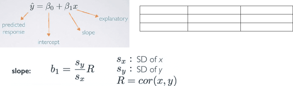
Estimating the regression parameters: slope
Ex: The standard deviation of % living in poverty is 3.1%, and the standard deviation of % of HS
graduates is 3.73%. Given that the correlation between these variables is -0.75, what is the slope
of the regression line for predicting the % living in poverty from % of HS graduates?
o sy = 3.1%; sx = 3.73%; R = -0.75
o b1 = (sy/sx) R = -0.62
Parameter
Point estimate
Intercept
β0
b0
Slope
β1
b1
o For each percentage point increase in HS graduation rate, we would expect the percentage
living in poverty to be lower on average by 0.62%.
o Be careful when interpreting the data, especially when it is an observational study – do not
use causal language
Estimating the regression parameters: intercept
o The least squares line always goes through (x-bar, y-bar)
o Rearranging the formula to – b0 = (y-bar) – b1(x-bar)
o Ex: Given that the average % living in poverty is 11.35% and the average % of HS graduates
is 86.01%, what is the intercept of the regression line for predicting % living poverty from
% HS graduates?
o b0 = 11.35 – (-0.62)(86.01) = 64.68
o States with no HS graduates are expected on average to have 64.68% of their residents
living below the poverty line.
▪ Important for putting together our linear model, but in context, not very realistic for
a state not to have any HS graduates
o We can write out our regression line model: (observed % in poverty) = 64.68 – 0.62(% of
HS grads)
o RECAP Intercept: When x = 0, y is expected to equal the intercept
▪ May be meaningless in context of the data and only serves to adjust the height of the
line
o Slope: For each unit increase in x, y is expected to be higher/lower on average by the slope
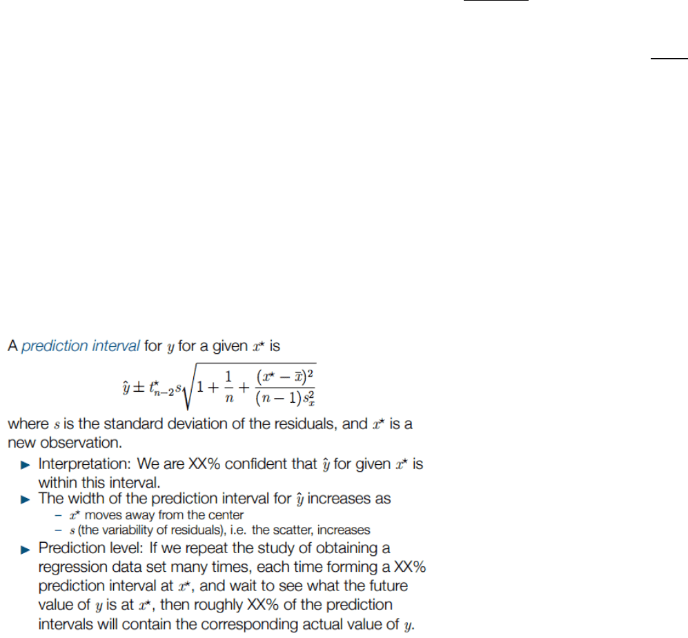
Part 2: (3) Prediction and Extrapolation
Prediction: using the linear model to predict the value of the response variable for a given value of
the explanatory variable
o Plugging in the x value to see what the resulting y value is
Ex: (observed % in poverty) = 64.68 – 0.62(% of HS grads)
o What is the predicted poverty rate in states where the HS graduation rate is 82%
o (observed % in poverty) = 64.68 – 0.62(82) = 13.84%
Extrapolation: applying a model estimate to values outside of the realm of the original data
o Sometimes the intercept might be an extrapolation
o We don’t know whether the line will continue to be linear, curve up, curve down beyond
the given data
o Thus, we do not want to conduct predictions on extrapolated data, since it would yield an
unreliable estimate
Document Summary
Correlation: measure of the strength of the linear relationship between two numerical variables: denoted as r. Difference between the observed and the predicted y. A measure for the best line: option 1: minimize the sum of magnitudes (absolute values of residuals, option 2: minimize the sum of squared residuals (least squares) Why least squares: a residual twice as large as another is more than twice as bad. Ex: the standard deviation of % living in poverty is 3. 1%, and the standard deviation of % of hs graduates is 3. 73%. % hs graduates: b0 = 11. 35 (-0. 62)(86. 01) = 64. 68, states with no hs graduates are expected on average to have 64. 68% of their residents living below the poverty line. Prediction: using the linear model to predict the value of the response variable for a given value of the explanatory variable: plugging in the x value to see what the resulting y value is.