CMSC 425 Lecture Notes - Lecture 3: Linear Interpolation, Inverse Kinematics, Shoulder Joint

15 May 2018
School
Department
Course
Professor
CMSC 425 Dave Mount & Roger Eastman
CMSC 425: Lecture 10
Skeletal Animation and Skinning
Reading: Chapt 11 of Gregory, Game Engine Architecture.
Recap: Last time we introduced the principal elements of skeletal models and discussed forward
kinematics. Recall that a skeletal model consists of a collection of joints, which have been
joined into a rooted tree structure. Each joint of the skeleton is associated with a coordinate
frame which specifies its position and orientation in space. Each joint can be rotated (subject
to sum constraints). The assignment of rotation angles (or generally rotation transformations)
to the individual joints defines the skeleton’s pose, that is, its geometrical configuration in
space. Joint rotations are defined relative to a default pose, called the bind pose (or reference
pose).
Last time, we showed how to determine the skeleton’s configuration from a set of joint angles.
This is called forward kinematics. (In contrast, inverse kinematics involves the question of
determining how to set the joint angles to achieve some desired configuration, such as grasping
a door knob.) Today we will discuss how animation clips are represented, how to cover these
skeletons with “skin” in order to form a realistic model, and how to move the skin smoothly
as part of the animation process.
Local and Global Pose Transformations: Recall from last time that, given a joint j(not the
root), its parent joint is denoted p(j). We assume that each joint jis associated with two
transformations, the local-pose transformation, denoted T[p(j)←j], which converts a point in
j’s coordinate system to its representation in its parent’s coordinate system, and the inverse
local-pose transformation, which reverses this process. (These transformations may be repre-
sented explicitly, say, as a 4 ×4 matrix in homogeneous coordinates, or implicitly by given a
translation vector and a rotation, expressed, say as a quaternion.)
Recall that these transformations are defined relative to the bind pose. By chaining (that is,
multiplying) these matrices together in an appropriate manner, for any two joints jand k,
we can generally compute the transformation T[k←j]that maps points in j’s coordinate frame
to their representation in k’s coordinate frame (again, with respect to the bind pose.)
Let M(for “Model”) denote the joint associated with the root of the model tree. We define
the global pose transformation, denoted T[M←j], to be the transformation that maps points
expressed locally relative to joint j’s coordinate frame to their representation relative to the
model’s global frame. Clearly, T[M←j]can be computed as the product of the local-pose
transformations from jup to the root of the tree.
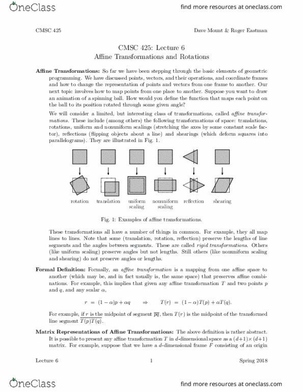
Meta-Joints: One complicating issue involving skeletal animation arises from the fact that dif-
ferent joints have different numbers of degrees of freedom. A clever trick that can be used
to store joints with multiple degrees of freedom (like a shoulder) is to break the into two or
more separate joints, one for each degree of freedom. These meta-joints share the same point
as their origin (that is, the translational offset between them is the zero vector). Each meta-
joint is responsible for a single rotational degree of freedom. For example, for the shoulder
one joint might handle rotation about the vertical axis (left-right) and another might handle
Lecture 10 1 Spring 2018

CMSC 425 Dave Mount & Roger Eastman
rotation about the forward axis (up-down) (see Fig. 1). Between the two, the full spectrum
of two-dimensional rotation can be covered. This allows us to assume that each joint has just
a single degree of freedom.
(a) (b)
Fig. 1: Using two meta-joints (b) to simulate a single joint with two degrees of freedom (a).
Animating the Model: There are a number of ways to obtain joint angles for an animation.
Here are a few:
Motion Capture: For the common motion of humans and animals, the easiest way to obtain
animation data is to capture the motion from a subject. Markers are placed on a
subject, who is then asked to perform certain actions (walking, running, jumping, etc.)
By tracking the markers using multiple cameras or other technologies, it is possible to
reconstruct the positions of the joints. From these, it is simple exercise in linear algebra
to determine the joint angles that gave rise to these motions.
Motion capture has the advantage of producing natural motions. Of course, it might be
difficult to apply for fictitious creatures, such as flying dragons.
Key-frame Generated: A design artist can use animation modeling software to specify
the joint angles. This is usually done by a process called key framing, where the artists
gives a detailed layout of the model at certain “key” instances in over the course of the
animation, called key frames. (For example, when animating a football kicker, the artist
might include the moment when the leg starts to swing forward, an intermediate point in
the swing, and the point at which the leg is at its maximum extension.) An automated
system can then be used to smoothly interpolate the joint angles between consecutive
key frames in order to obtain the final animation. (The term “frame” here should not
be confused with the use of term “coordinate frame” associated with the joints.)
Goal Oriented/Inverse kinematics: In an ideal world, an animator could specify the de-
sired behavior at a high level (e.g., “a character approaches a table and picks up a
book”). Then the physics/AI systems would determine a natural-looking animation to
achieve this. This is quite challenging. The reason is that the problem is under-specified,
and it can be quite difficult to select among an infinite number of valid solutions. Also,
determining the joint angles to achieve a particular goal reduces to a complex nonlinear
optimization problem.
Lecture 10 2 Spring 2018

CMSC 425 Dave Mount & Roger Eastman
Representing Animation Clips: In order to specify an animation, we need to specify how the
joint angles or generally the joint frames vary with time. This can result in a huge amount
of data. Each joint that can be independently rotated defines a degree of freedom in the
specification of the pose. For example, the human body has over 200 degrees of freedom!
(It’s amazing to think that our brain can control it all!) Of course, this counts lots of fine
motion that would not normally be part of an animation, but even a crude modeling of just
arms (not including fingers), legs (not including toes), torso, neck involves over 20 degrees of
freedom.
As with any digital signal processing (such as image, audio, and video processing), the stan-
dard approach for efficiently representing animation data is to first sample the data at suf-
ficiently small time intervals. Then, use some form of interpolation technique to produce a
smooth reconstruction of the animation. The simplest manner to interpolate values is based
on linear interpolation. It may be desireable to produce smoother results by applying more
sophisticated interpolations, such as quadratic or cubic spline interpolations. When dealing
with rotated vector quantities, it is common to use spherical interpolation.
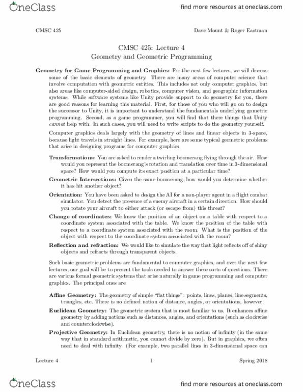
In Fig. 2 we give a graphical presentation of a animation clip. Let us consider a fairly general
set up, in which each pose transformation (either local or global, depending on what your
system prefers) is represented by a 3-element translation vector (x, y, z) indicating the joint
frame’s position and a 4-element quaternion vector (s, t, u, v) to represent the frame’s rotation.
Each row of this representation is a sequence of scalar values, and is called a channel.
Time samples
01234567
x
y
z
s
t
u
v
Joint 0
x
y
z
s
t
u
v
Joint 1
Time
T0,x
T0
Q0
T1
Q1
Linear interpolation
Frame rate
Time samples
01234567
x
y
z
s
t
u
v
Joint 0
x
y
z
s
t
u
v
Joint 1
Time
T0,x
T0
Q0
T1
Q1
Linear interpolation
Frame rate
Meta channels Event triggers
Left footstep Right footstep
Camera motion
Fig. 2: An uncompressed animation stream.
It is often useful to add further information to the animation, which are not necessarily related
to the rendering of the moving character. Examples include:
Event triggers: These are discrete signals sent to other parts of the game system. For
example, you might want a certain sound playback to start with a particular event (e.g.,
footstep sound), a display event (e.g., starting a particle system that shows a cloud
Lecture 10 3 Spring 2018