CMSC 425 Lecture Notes - Lecture 6: Homogeneous Coordinates, Rotation Matrix, Unit Vector

15 May 2018
School
Department
Course
Professor

CMSC 425 Dave Mount & Roger Eastman
CMSC 425: Lecture 6
Affine Transformations and Rotations
Affine Transformations: So far we have been stepping through the basic elements of geometric
programming. We have discussed points, vectors, and their operations, and coordinate frames
and how to change the representation of points and vectors from one frame to another. Our
next topic involves how to map points from one place to another. Suppose you want to draw
an animation of a spinning ball. How would you define the function that maps each point on
the ball to its position rotated through some given angle?
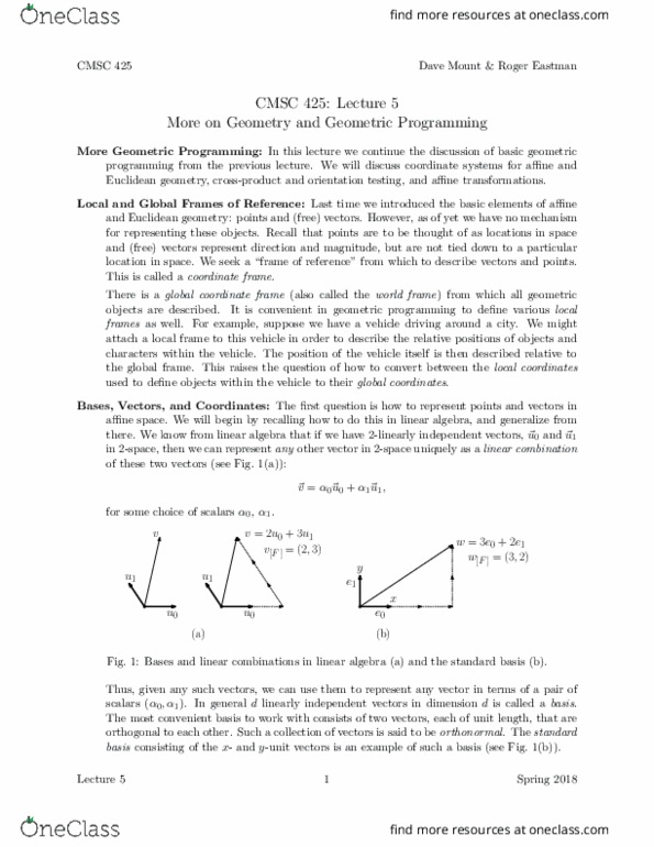
We will consider a limited, but interesting class of transformations, called affine transfor-
mations. These include (among others) the following transformations of space: translations,
rotations, uniform and nonuniform scalings (stretching the axes by some constant scale fac-
tor), reflections (flipping objects about a line) and shearings (which deform squares into
parallelograms). They are illustrated in Fig. 1.
rotation translation uniform
scaling nonuniform
scaling reflection shearing
Fig. 1: Examples of affine transformations.
These transformations all have a number of things in common. For example, they all map
lines to lines. Note that some (translation, rotation, reflection) preserve the lengths of line
segments and the angles between segments. These are called rigid transformations. Others
(like uniform scaling) preserve angles but not lengths. Still others (like nonuniform scaling
and shearing) do not preserve angles or lengths.
Formal Definition: Formally, an affine transformation is a mapping from one affine space to
another (which may be, and in fact usually is, the same space) that preserves affine combi-
nations. For example, this implies that given any affine transformation Tand two points p
and q, and any scalar α,
r= (1 −α)p+αq ⇒T(r) = (1 −α)T(p) + αT (q).
For example, if ris the midpoint of segment pq, then T(r) is the midpoint of the transformed
line segment T(p)T(q).
Matrix Representations of Affine Transformations: The above definition is rather abstract.
It is possible to present any affine transformation Tin d-dimensional space as a (d+1)×(d+1)
matrix. For example, suppose that we have a d-dimensional frame Fconsisting of an origin
Lecture 6 1 Spring 2018

CMSC 425 Dave Mount & Roger Eastman
point F.Oand basis vectors F.~e0through F.~ed−1. To express Tin the form of a matrix,
we determine where each of these frame components is mapped, and then generate a matrix
whose first dcolumns are the images of the basis vectors and whose last component is the
image of the origin point. (It follows, therefore, that the last row of such a matrix must be
(0,...,0,1), because the basis vectors must map to vectors, which must end in 0 according
to the rules of affine homogeneous coordinates, and the origin point maps to a point, which
must end in 1 by these same rules.)
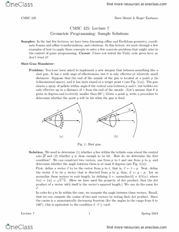
For example, consider the affine transformation (in 2-dimensional space) shown in Fig. 2,
which rotates by 30◦degrees about the origin and translates 2 units to the right and 1 unit
up. This transformation maps the origin F.Oto the point Owith homogeneous coordinates
(2,1,1), the x-axis is mapped to the vector ~u0= (cos 30◦,sin 30◦,0) = (√3/2,1/2,0), and
the y-axis is mapped to (−sin 30◦,cos 30◦,0) = (−1/2,√3/2,0). By forming a matrix whose
columns are consist of ~u0,~u1, and O, as shown in the figure.
FO
F~e1
F~e0
O= (2,1,1)
~u1=
−1
2,√3
2,0
~u0=
√3
2,1
2,0
√3
2
1
2
0
√3
2
1
2
0
1
2
1
G
Fig. 2: Generating a homogeneous matrix for an affine transformation.
Let’s consider a number of examples representing affine transformations in 3-dimensional
space by 4 ×4 matrices. (The two dimensional cases can be extracted by just ignoring the
rows and columns for the z-coordinates.)
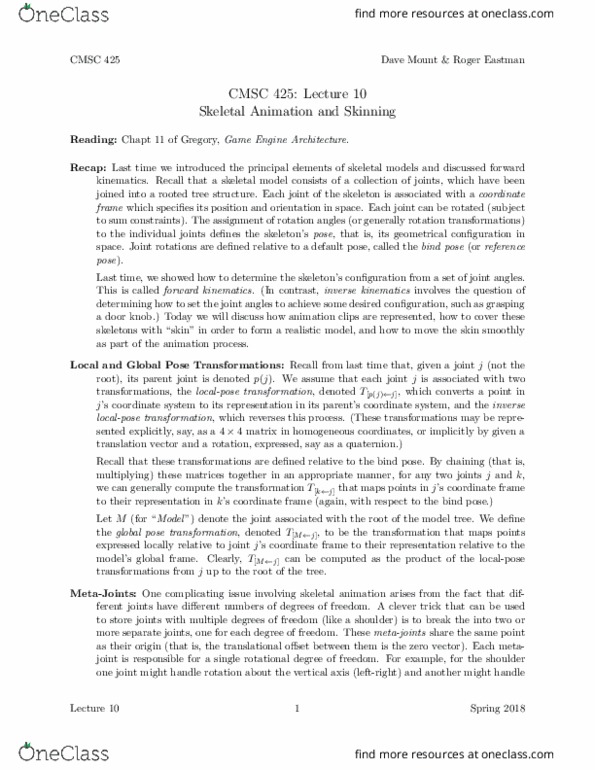
Translation: Translation by a fixed vector ~v maps any point pto p+~v. Note that, since
free vectors have no position in space, they are not altered by translation (see Fig. 3(a)).
Suppose that relative to the standard frame, v[F]=(αx, αy, αz,0) are the homogeneous
coordinates of ~v. The three unit vectors are unaffected by translation, and the origin is
mapped to O+~v, whose homogeneous coordinates are (αx, αy, αz,1). Thus, by the rule
given earlier, the homogeneous matrix representation for this translation transformation
is
T(~v) =
1 0 0 αx
0 1 0 αy
0 0 1 αz
0 0 0 1
.
Scaling: Uniform scaling is a transformation which is performed relative to some central
fixed point. We will assume that this point is the origin of the standard coordinate
frame. (We will leave the general case of scaling about an arbitrary point in space as an
exercise.) Given a scalar β, this transformation maps the object (point or vector) with
coordinates (αx, αy, αz, αw) to (βαx, βαy, βαz, αw) (see Fig. 3(b)).
In general, it is possible to specify separate scaling factors for each of the axes. This
is called nonuniform scaling. The unit vectors are each stretched by the corresponding
Lecture 6 2 Spring 2018

CMSC 425 Dave Mount & Roger Eastman
o e0
e1
o+ve0
e1
o e0
e1
2e0
2e1
o
translation by v
uniform scaling by 2
(a) (b)
reflection about the y-axis
(c)
o e0
e1
o e0
e1
Fig. 3: Derivation of transformation matrices.
scaling factor, and the origin is unmoved. Thus, the transformation matrix has the
following form:
S(βx, βy, βz) =
βx0 0 0
0βy0 0
0 0 βz0
0 0 0 1
.
Observe that both points and vectors are altered by scaling.
Reflection: In its most general form, a reflection in the plane is given a line and maps points
by flipping the plane about this line. A reflection in 3-space is given a plane, and flips
points in space about this plane. In this case, reflection is just a special case of scaling,
but where the scale factor is negative. A common simple version of this is when the plane
about which the reflection is performed is one of the coordinate planes (corresponding
to x= 0, y= 0, or z= 0).
For example, to reflect points about the yz-coordinate plane (that is, the plane x= 0),
we can scale the x-coordinate by −1 (see Fig. 3(c)). Using the scaling matrix above, we
have the following transformation matrix:
Fx=
−1 0 0 0
0 1 0 0
0 0 1 0
0 0 0 1
.
The cases for the other two coordinate frames are similar. Reflection about an arbitrary
line (in 2-space) or a plane (in 3-space) is left as an exercise.
Rotation: In its most general form, rotation is defined to take place about some fixed point,
and around some fixed vector in space. We will consider the simplest case where the fixed
point is the origin of the coordinate frame, and the vector is one of the coordinate axes.
There are three basic rotations: about the x,yand z-axes. In each case the rotation
is counterclockwise through an angle θ(given in radians). The rotation is assumed to
be in accordance with a right-hand rule: if your right thumb is aligned with the axes of
rotation, then positive rotation is indicated by the direction in which the fingers of this
hand are pointing. To produce a clockwise rotation, simply negate the angle involved.
Consider a rotation about the z-axis. The z-unit vector and origin are unchanged.
The x-unit vector is mapped to (cos θ, sin θ, 0,0), and the y-unit vector is mapped to
Lecture 6 3 Spring 2018
Document Summary
A ne transformations: so far we have been stepping through the basic elements of geometric programming. We have discussed points, vectors, and their operations, and coordinate frames and how to change the representation of points and vectors from one frame to another. Our next topic involves how to map points from one place to another. Suppose you want to draw an animation of a spinning ball. We will consider a limited, but interesting class of transformations, called a ne transfor- mations. These include (among others) the following transformations of space: translations, rotations, uniform and nonuniform scalings (stretching the axes by some constant scale fac- tor), re ections ( ipping objects about a line) and shearings (which deform squares into parallelograms). 1. rotation translation uniform scaling nonuniform scaling re ection shearing. These transformations all have a number of things in common. For example, they all map lines to lines.