STAT 1450 Final: Chapter 15 Notes - Sampling Distributions

17 Sep 2020
School
Department
Course
Professor
Chapter 15, page 1
STAT 1450 COURSE NOTES – CHAPTER 15
SAMPLING DISTRIBUTIONS
Connecting Chapter 15 to our Current Knowledge of Statistics
Chapters 1 9 focused a lot on data analysis and data collection.
Chapter 12 introduced us to probability.
A primary tenet was that if we obtained a representative sample of some phenomenon,
then the rules of probability would allow us to generalize information from our random
sample to make a statement about our population of interest.
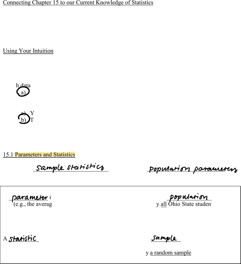
Using Your Intuition
Suppose you generate a random sample of 9 values (0 to 10); yielding an average of 6.7.
The instructor then collects your average along with the averages of 4 other students.
The instructor cme he aeage f he aeage.
Which data set would you expect to have a larger range? ____________
a) Your sample of 9 values or b) The instructor e f 5 averages
Then, which would you expect to have a greater likelihood of occurring? ___________
a) You obtaining an average greater than 8.
b) The instructor obtaining an average of averages greater than 8
In this chapter we will support your intuition
with rules that describe how sample statistics behave.
15.1 Parameters and Statistics
We will use ____________________________ to estimate __________________________.
From Chapter 8.
A _____________ is a number that describes a characteristic of the _______________
(e.g., the average number of text messages sent yesterday by all Ohio State students).
Often the value of a parameter is unknown because we cannot examine the entire population.
A ____________ is a number that can be computed from the __________ data.
(e.g., the average number of text messages sent yesterday by a random sample of OSU juniors).
samplestatistics populationparameters
parameter population
statistic sample
Chapter 15, page 2
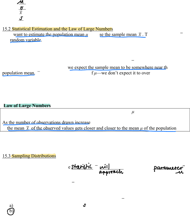
Notation:
___
population mean
___
population standard deviation
x
sample ________
___
sample standard deviation
15.2 Statistical Estimation and the Law of Large Numbers
If we want to estimate the population mean μ, we use the sample mean
x
. The sample mean
x
is a random variable. We learned in Chapter 12 that each random variable has a probability
model which tells us the values the random variable can take and the probability that it takes on
these values.
Hee an ineeing hgh: he babili ha he amle mean
x
is exactly equal to the
population mean μ is 0. However, we expect the sample mean to be somewhere near the
population mean.
x
is an unbiased estimator of μe dn eec i e- or underestimate
the population mean.
And, as we sample more and more individuals from the population, we expect the sample mean
to get closer to the population meanthis is a Law of Large Nmbe
Law of Large Numbers
Draw observations at random from any population with finite mean μ.
As the number of observations drawn increases,
the mean
x
of the observed values gets closer and closer to the mean μ of the population.
Check out Example 15.3 on page 347 of the book for a nice example and graphic of the law of
large numbers.
15.3 Sampling Distributions
The law of large numbers says,
sample enough individuals and the _________
x
__________ the unknown ____________.
Typically we take just one sample and then generalize to the population as a whole. Before we
do that, we need to understand how
x
behaves. This can be done through simulation
(see Example 15.4 on page 350).
Poll: As the sample size increases, the variability of the mean,
x
, of the observed values ______.
a) increases.
b) decreases.
no
s
statistic nitproach parameter
O
Document Summary
Connecting chapter 15 to our current knowledge of statistics. Chapters 1 (cid:177) 9 focused a lot on data analysis and data collection. A primary tenet was that if we obtained a representative sample of some phenomenon, then the rules of probability would allow us to generalize information from our random sample to make a statement about our population of interest. Suppose you generate a random sample of 9 values (0 to 10); yielding an average of 6. 7. The instructor then collects your average along with the averages of 4 other students. The instructor c(cid:82)m(cid:83)(cid:88)(cid:87)e(cid:86) (cid:87)he (cid:181)a(cid:89)e(cid:85)age (cid:82)f (cid:87)he a(cid:89)e(cid:85)age(cid:86). (cid:182) Which data set would you expect to have a larger range: your sample of 9 values or, the instructor(cid:182)(cid:86) (cid:86)e(cid:87) (cid:82)f 5 averages. Then, which would you expect to have a greater likelihood of occurring: you obtaining an average greater than 8, the instructor obtaining an average of averages greater than 8 (cid:171)