STA 101 Chapter Notes - Chapter Unit 4: Statistical Hypothesis Testing, Percentile, Stellar Population

10 May 2018
School
Department
Course
Professor

Unit 4: Inference for Numerical Variables
Part 1: (1) t-distribution
What purpose does a large sample size?
o As long as observations are independent, and the population distribution is not extremely
skewed, a large sample would ensure that
▪ The sampling distribution of the mean is nearly normal
▪ The estimate of the standard error is reliable s/√n
What if we have a small sample size?
o Okay, then how do we address the uncertainty associated with the standard error?
▪ T-distribution!
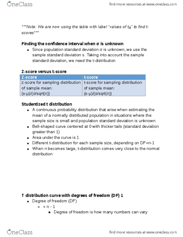
T distribution
o When σ is unknown (almost always), use the t-distribution to address the uncertainty of
the standard error estimate
o Bell shaped but thicker tails than the normal
▪ Observations are more likely to fall beyond 2 SDs from the mean
▪ Confidence intervals constructed under the t-distribution will be wider
▪ Extra thick tails helpful for mitigating the effect of a less reliable estimate for the
standard error of the sampling distribution
o Always centered at 0 (like the normal dist.)
o Has one parameter: degrees of freedom (df) – determines the thickness
▪ Compare to normal dist., which has two parameters – SD and mean
▪ What happens to the shape of the t-distribution as degrees of freedom increases?
• As df increases, the shape of the t-distribution approaches the normal
distribution
T statistic is for inference of a mean when σ is unknown, which is almost always
o Calculated the same way
▪ T = (obs. – null)/SE
o P-value (same definition)
Find the following probabilities. Suppose you have a two-sided hypothesis test and your test
statistic is 2. Under which of these scenarios would you be able to reject the null hypothesis at the
5% significance level?
o P (|Z| > 2) = 0.0455 – REJECT
o P (|tdf=50| > 20) = 0.0509 – FAIL TO REJECT
o P (|tdf=10| > 20) = 0.0734 – FAIL TO REJECT
o As the df decreases (t-distribution becomes more conservative), we become less likely to
reject the null hypothesis
Part 1: (2) Inference for a Mean
Ex: Playing a computer game during lunch affects memory for lunch, and later snack intake
o Researchers assessing relationship between distraction and recall of food consumer and
snacking
o Sample – 44 patient (22 men and 22 women)
o Randomized into two groups – 1) play solitaire while eating and 2) eat lunch without
distractions – both groups were offered biscuits to snack on after lunch
Biscuit intake
x-bar
S
N
Solitaire
52.1 g
45.1 g
22
No distraction
27.1 g
26.4 g
22
Estimating the mean
o Confidence of the form Point estimate ± margin of error
find more resources at oneclass.com
find more resources at oneclass.com

o x̄ ± t*df(SEx̄ ) = x̄ ± t*df(s/√n) = x̄ ± t*n-1(s/√n)
o Degrees of freedom for t-statistic for inference on one sample mean df = n – 1
Estimating the mean for the above example
o x̄ ± t*df(SEx̄ ) = (32.1, 72.1)
o We are 95% confident that distracted eaters consume between 32.1 to 72.1 grams of
snacks post-meal.
Ex: Suppose the suggested serving size of these biscuits is 30 g. Do these data provide convincing
evidence that the amount of snacks consumed by distracted eaters post-lunch is different from the
suggested serving size?
o 0.02 < p-value < 0.05
o We reject the null hypothesis (which agrees with the result of the confidence interval)
Conditions
o Independent observations
▪ Random assignment
▪ 22 < 10% of all distracted eaters
o Sample size/skew
▪ We don’t have a visualization of the population distribution, so we will look at the
sample distribution
• There is a natural boundary at 0 grams
• Data is right-skewed
Part 1: (3) Inference for comparing two independent means
DF for t statistic for inference on difference of two means df = min (n1 – 1, n2 – 1)
Refer to the distracted eaters study
Confidence interval for difference between independent means
o Correct interpretation – We are 95% confident that those who eat with distractions
consume 1.83 g and 48.17 g more snacks than those who eat without distractions, on
average
o Incorrect – We are 95% confident that the difference between the average snack
consumption of those who eat with and without distractions is between 1.83 g and 48.17 g.
Using hypothesis testing, the p-value is between 0.2 and 0.5
We reject the null hypothesis
Conditions for inference for comparing two independent means:
o Independence:
▪ Within groups: sampled observations must be independent
• Random assignment
• If sampling without replacement, n < 10% of population
▪ Between groups: the two groups must be independent of each other (non-paired)
o Sample size/skew: The more skew in the population distributions, the higher the sample
size needed
Part 1: (4) Inference for comparing two paired means
Analyzing paired data
o When two sets of observations have this special correspondence (not independent), they
are said to be paired
find more resources at oneclass.com
find more resources at oneclass.com