COMMERCE 3QA3 Chapter Notes - Chapter 8: Minimax, Shape Parameter, Cheat Sheet

4 Jun 2018
School
Department
Course
Professor

Decision making under risk – ≥2 stages Lectures 22-27 – Ch. 8 (Decision analysis) – part 2of 2 page 14
5iii) Decision making under risk— ≥ 2 stages: decision trees <click here to go to the podcast>
The manager can list the possible future outcomes and can estimate the probability that a
specific outcome will occur. Two or more decisions are made; usually at different times (or
stages). A decision tree is needed to depict and analyze the problem. One of three decision-
making criteria is used to make a decision: EMV, EOL, EU.
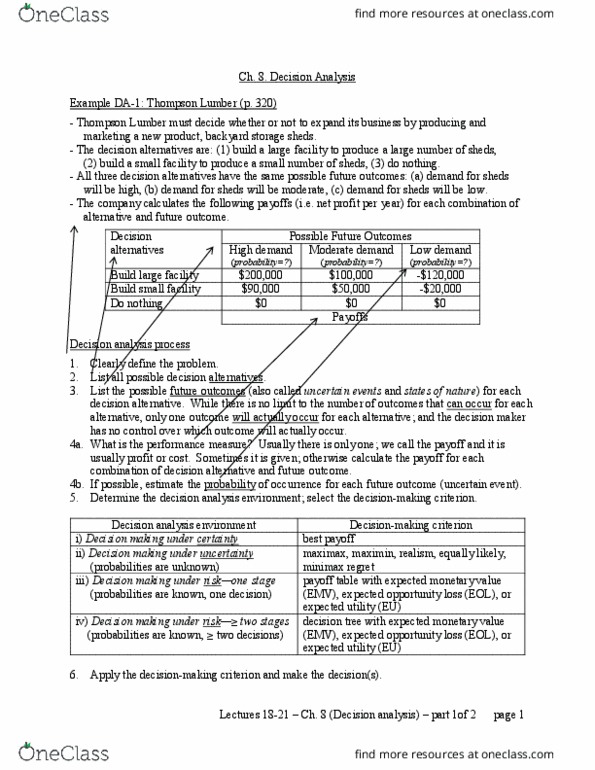
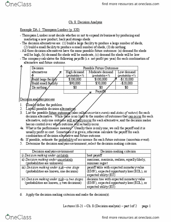
Example DA-1: Thompson Lumber (continued)
Decision
alternatives
Payoffs for each Possible Future Outcome
(probability)
Expected payoff, EMV
High demand
(0.3)
Moderate demand
(0.5)
Low demand
(0.2)
Build large facility
$200k
$100k
-$120k
200×0.3 +100×0.5 – 120×0.2 = 86k
Build small facility
$90k
$50k
-$20k
90×0.3 + 50×0.5 – 20×0.2 = 48k
Do nothing
$0
$0
$0
$0
Best payoff for an
outcome
$200k
$100k
$0
EVwPI =
200×0.3 +100×0.5 + 0×0.2 = 110k
The best EMV is $86,000. The decision is: build a large facility.
EVPI = EVwPI – best EMV = 110k – 86k = $24,000
Although this is a one stage problem (i.e. one decision at one point of time) and, therefore, we
use a payoff table (as shown), we can also draw a decision tree for this problem.
Decision trees
1. Draw the tree: Any decision analysis problem can be presented graphically as a decision tree.
A decision tree presents the decision alternatives and future outcomes in a sequential (i.e. time)
manner using decision nodes with arcs, outcome nodes with arcs, and end nodes with payoffs.
□ = decision node. The arcs (or lines) originating from a decision node represent decision
alternatives available to the decision maker at that point in time. Of these, the decision maker
must select only one alternative. Most trees begin with a decision node.
○ = outcome (or event) node. The arcs (lines) originating from an outcome node represent all
outcomes that could occur at that node. Each outcome has a probability. Only one outcome
will actually occur. The decision maker has no control over which outcome will occur.
◄ = end (or terminal) node. Each path of decision alternatives and outcomes in the decision
tree ends at an end node. The payoff (usually the monetary value, MV) at the end node is the
result of the decision alternatives and outcomes on that path.
2. Fold back the tree: Decision trees are analyzed by a process called folding back the tree: ‘back’
means the end of the tree back to the front of the tree , ‘folding’ means we follow two rules.
1. At each outcome node, we calculate the expected payoff (usually the expected monetary
value, EMV or the expected utility, EU).
2. At each decision node, we select the alternative with the best EMV or EU.
find more resources at oneclass.com
find more resources at oneclass.com

Decision making under risk – ≥2 stages Lectures 22-27 – Ch. 8 (Decision analysis) – part 2of 2 page 15
Example DA-1: (continued)
- Drawing the tree:
Fig. 8.1, p. 331
0 1 year 2 years Time
- Folding back the tree:
The tree in Fig. 8.1 above is equivalent to the following tree.
The tree in Fig. 8.2 above is equivalent to the following tree.
0 1 year 2 years Time
- Result: EMV = $86k for the ‘Large Plant’ alternative is the best. So the best decision at the
Decision Node at time 0 is to build a large plant. From Fig 8.2 after one year the plant will be
finished and demand will begin. At the end of two years the demand will have been high,
moderate, or low and the actual payoffs will be one of $200k, $100k, or -$120k, respectively.
◄
◄
◄
◄
(0.30)
(0.50)
(0.20)
Probability
0 1 year 2 years Time
(0.30)
(0.50)
(0.20)
◄
◄
◄
◄
◄
◄
◄
◄
◄
◄
These values are the same as in the
payoff table on the previous page
(1.00)
(1.00)
$86k
find more resources at oneclass.com
find more resources at oneclass.com

Decision making under risk – ≥2 stages Lectures 22-27 – Ch. 8 (Decision analysis) – part 2of 2 page 16
Example DA-4: Folding back another decision tree
Consider the following decision tree for a two-stage (i.e. two decision) problem (which we will
study later). Fold back the decision tree (i.e. apply the two rules from right to left, , in the tree).
Decision tree for decision problem:
Tree 1 is equivalent to:
-
-
(0.30)
(0.50)
(0.20)
EMV = 200×0.3 + 100×0.5 – 120×0.2 = $86k
EMV = 90×0.3 + 90×0.5 – 20×0.2 = $48k
EMV = $0k
EMV = 196×0.509 + 96×0.468 – 124×0.023 = $141.84k
EMV = 86×0.509 + 46×0.468 – 24×0.023 = $64.75
EMV = - $4k
EMV = 196×0.023 + 96×0.543 – 124×0.434 = $2.82k
EMV = 86×0.023 + 46×0.543 – 24×0.434 = $16.54
EMV = - $24k
0 3 months 1 year 2 years Time
0 3 months 1 year Time
Tree 1
Tree 2
(0.468)
(0.468)
$141,840
find more resources at oneclass.com
find more resources at oneclass.com