ECO 305 Study Guide - Quiz Guide: Isoquant, Diminishing Returns, Production Function


Prof. Bucci
ECO 305
25 October 2017
Problem Set #4
1. How is an isoquant map like an indifference map? In what important ways are they different?
Isoquants and indifference curves are downward sloping, they cannot cross and you get more
utility/output as you get further away from the origin. Isoquant maps are constructed to
measure something cardinal while indifference maps are constructed to measure something
ordinal.
2. Graph the short run total product curve for the following production functions if Kapital is fixed
at K = 4.
a. Q = 2K + 3L = 2(4) + 3L = 8+3L
b. Q = K2 L2 = (4)2L2 = 16L2
3. Do the production functions in question 2 obey the law of diminishing returns? Explain why or
why not.
The production function in A has a constant marginal product of labor for all levels of labor input,
and B has an increasing marginal product of labor for all levels of labor input. So neither
production function obeys the law of diminishing returns.
4. Do the production functions in question 2 exhibit constant, increasing or decreasing returns to
scale? Show and explain.
Function A exhibits constant returns to scale while B exhibits increasing returns to scale. You can
tell by the slopes of the functions in the graphs.
5. For the production functions in question 2, write an expression for MPK, MPL, and MRTS for
each production function.
a. MRTS= -12/4, MPK= 1+3L, MPL= 2K+3
b. MRTS= -48, MPK= KL2, MPL= K2L
4 L
8 20 K
16 64 144 K
1 2 3 L
find more resources at oneclass.com
find more resources at oneclass.com
Document Summary
Isoquants and indifference curves are downward sloping, they cannot cross and you get more utility/output as you get further away from the origin. The production function in a has a constant marginal product of labor for all levels of labor input, and b has an increasing marginal product of labor for all levels of labor input. Function a exhibits constant returns to scale while b exhibits increasing returns to scale. A competitive firm has the cost structure given in the following table. Graph the marginal cost, average variable cost and average total cost curves. Calculate profit and show it on your graph. Plugging this in you get the equation; profit =(p-atc)q= 4(32-26)4 = : a firm in a competitive industry has total cost curve given by tc = 30 + 0. 2 q2 5q. The corresponding marginal cost mc = 0. 4q- 5. Cost =27. 5*6-[0. 2(27. 5) 2 5(27. 5) + 30] = 121. 2. With a positive profit, the firm should continue operating.