SOAN 3120 Study Guide - Midterm Guide: Scatter Plot, Explained Variation, Standard Deviation

22 Oct 2016
School
Department
Course
Professor

SOAN 3120
Midterm 2 Review
Chapter 5: Simple Regression
Regression Line
• A straight line that describes how a response variable y changes as an explanatory variable x changes
• We use a regression line to predict the values of y for a given value of x when we believe the relationship
between y and x is linear
• The slope is the rate of change in the response
• You cant say how important a relationship is by looking at the size of the slope of the regression line
Least Squares Regression
• Least squares regression line: of y on x is the line that makes the sum of the squares of the vertical distances
of the data points from the line as small as possible
• We give the equation for the least squares regression line in terms of the means and standard deviations of
the two variables and the correlation between them
• Because of the scatter of points about the line, the predicted response will usually not be exactly the same
and the actual observed response
• Plotting for the purpose of prediction
• Summarizes the linear relationship between x and y
• Represented by the equation y= n+b(x)
o N/a = Y intercept, the y value when x is 0
o B = Slope, the change in y when x increases by 1 (if slope is positive then y increases with x, if slope is
negative then y decreases as x increases)(slope is the rate at which the predicted response y changes
along the line as the explanatory x changes)
o If the slope (b) is 0 (a horizontal line), then, there is no change in y as x changes
o Least squares regression allows us to predict values of y for specific values of x
o Residual: difference between what is observed and what is predicted (to calculate the value for
residual, we take the observed value – the predicted value)→ we want a line that makes the residual
as small as possible (closest to 0)
o Least squares regression find the line with the smallest possible residuals
o Y with a hat (^) used to predict values of y (y hat = a + b (x)
where b = rx sx
sy
o In order to calculate slope, we need to know the standard deviations for x and y
o To plot the regression line one the scatter plot find 2 points on the line (y intercept and mean of x
and y are always on the line)
o A good regression line makes the vertical distances of the points from the line as small as possible
(the sum of the squares of distances)
Facts about Least-Squares Regression
1. The distinction between explanatory and response variables is essential in regression (least squares
regression makes the distances of the data points from the line small only in the y direction, if reverse the
roles of the two variables, we get a different least-squares regression line)
find more resources at oneclass.com
find more resources at oneclass.com
2. There is a close connection between correlation and the slope of the least-squares line (the slope and the
correlation always have the same sign (-, +), along the regression line, a change of one standard deviation in
x corresponds to a change of r standard deviations in y
3. The least-squares regression line always passes through the point (x, y) on the graph of y against x
4. The correlation r describes the strength of a straight line relationship, in the regression setting the square
of the correlation (r squared) is the fraction of the variation in the values of y that is explained by the least-
squares regression of y on x
You can find a regression line for any relationship between two quantitative variables, but the
usefulness of the line for prediction depends on the strength of the linear relationship→ when you
see a correlation, square it to get a better feel for the strength of the relationship
• The correlation (r) is the slope of the least-squares regression line when we measure both x
and y in standardized units
Residuals
• A residual is the difference between an observed value of the response variable and the value predicted by
the regression line
• The residual is negative when the data point lies below the regression line
• The residual is positive when the data point lies above the regression line
• Examining the residuals helps us to assess how well the line describes the data
• The mean of the least-squares residual is always zero
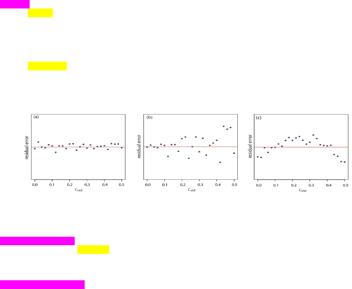
• A residual plot is a scatter plot of the regression residuals against the explanatory variable, residual plots
help us to assess how well a regression line fits the data
• A residual plot magnifies the deviations of the points from the line and makes it easier to see unusual
observations and patterns
• Predictions of the response will be more precise for smaller values of the explanatory variable,
where the response shows less variability about the line
• A) Unstructured horizontal band, centered as 0
• B) Curved pattern, indicates the relationship between the response and the explanatory variable is curved
rather than linear
• C) Fan shaped pattern, shows that the variation of the response about the least-squares line increases as the
explanatory variable increases
Influential Observations
• An observation is influential for a statistical calculation if removing it would markedly change the result of
the calculation
• Changes in a calculation that differ by a factor of 1.5 or more are often influential
• In the regression setting however, not all outliers are influential
Correlation and Regression
find more resources at oneclass.com
find more resources at oneclass.com

• The correlation ® and the slope (b) are similar in certain respects and different in others:
o When y=0 (there is no linear relationship between y and x), then b=0 as well
o If x and y are standardized variables (sx = sy = 1) then b=y
o Unlike r, the slope (b) does depend on the which variable is treated as explanatory and which is
response
If x is regressed on y (x becomes the response variable) b = r sx
sy
o Unless r=1, this regression line is different from b (slope)
o The squared correlation expressed the explained variation as a fraction of the total variation of ys
R squared = explained variation (this gives us the strength of the association)
total variation
• When there is a perfect linear relationship between x and y, the residuals are all zero, and r squared equals
1 (meaning that 100% of the variation is explained)
• When there is no linear relationship between x and y, the explained variation is zero and r squared is zero
Potential Problems
• In regression analysis, an outlier is a point whose y value is unusual compared to other points with similar x
values
• Points with unusual x values can also markedly enter the regression line
• Outliers, influential data and other problems in regression analysis can be detected in the scatter plot of y
against x → and are often seen more clearly in plots of residual against y
Anscombes Regression Data sets
• Four of the same data sets (completely differing values (means, medians, standard deviations)—all have the
same correlation (r)
• The regression line is different on all data sets, despite the correlations being the same
Cautions with Interpretation
• Correlation and regression lines describe only linear relationships (you can calculate it for any but it is only
useful for linear relations)
• Correlation and least-squares regression lines are not resistant (always plot and look for influential
observations)
• Ecological correlation: A correlation based on averages rather than individuals (e.g. average income and
correlation)
• Extrapolation: Not safe to use a regression line for prediction outside of the range of explanatory x-values
observed in the data e.g. child’s height—extending the line is foolish)
• Lurking variables: A variable that is not among the explanatory or response variables in a study and yet
may influence the interpretation of relationships—explanatory variables omitted from the analysis can
have an important effect on the relationship between x and y (e.g. family background is a lurking variable
that explains why test scores are related to experience with music)
• Association is not causation → an association is explained by lurking variables
Chapter 6: Contingency Tables
• Two-way table: describes two categorical variables (sex and education)
• Row variable: each row in the table describes a combination of sex and education level
• Column variable: each column describes one choice
Marginal Distributions
find more resources at oneclass.com
find more resources at oneclass.com
Document Summary
Influential observations: an observation is influential for a statistical calculation if removing it would markedly change the result of the calculation, changes in a calculation that differ by a factor of 1. 5 or more are often influential. In the regression setting however, not all outliers are influential. R squared = explained variation (this gives us the strength of the association) total variation: when there is a perfect linear relationship between x and y, the residuals are all zero, and r squared equals. 1 (meaning that 100% of the variation is explained: when there is no linear relationship between x and y, the explained variation is zero and r squared is zero. Table formatting: calculate percentages within categories of the explanatory variable to make comparisons between them. Include the total counts on which percentages are based. If education wholly mediates the relationship, it should disappear when education is held constant.