STAT1008 Study Guide - Final Guide: Central Limit Theorem, Confidence Interval, Normal Distribution


Normal Distribution
Density Curve
• A density curve is a theoretical model to describe a variable's distribution.
• Think of a density curve as an idealised histogram, where:
1. The total area under the curve is equal to 1.
2. The area over any interval is the proportion of the distribution in that interval.
Normal Distribution
• A normal distribution has a symmetric bell-shaped density curve.
• Two features distinguish one normal density from another:
1. The mean is its centre of symmetry (μ).
2. The standard deviation controls it spread (σ).
• Notation: X~N(μ,σ)
Normal Density Curve
• A normal distribution follows a bell-shaped curve.
• We use the two parameters mean, μ, ad stadard deiatio, σ, to
distinguish one normal curve from another.
• For a shorthand we often use the otatio N μ, σ to speify that a distriutio is oral N.
Graph of a Normal Density Curve
• The graph of a oral desity ure N μ, σ is a ell-shaped curve which:
o Is etred at the ea μ
o Has a horizontal scale such that 95% of the area under the curve falls within two SDs
of the ea ithi μ ± σ.
Standard Normal N(0, 1)
• Stadard Noral: μ = ad σ = → Z ~ N (0, 1).
• To convert any X~N(μ, σ to )~N,, use the z-score: Z = (X-μ/σ.
• To oert fro ) ~ N , to ay X ~ N μ, σ, e reerse the stadardisatio ith: X = μ + )σ.
Standardising
• The process of converting any Normal random variable to a Standard Normal Random Variable.
• If X~N(μ,σ²), then use the linear transformation below: Z= (X – μ/ σ ~ N,.
• For Z~N(0,1), values for Pr(Z<z) are available in tables.
• Symmetry → P(Z<-a) = P(Z>a).
• Total area under curve is 1, total area under each half of curve is 0.5, i.e. P(Z<0) = P(Z>0) = 0.5.
• If we are interested in a point so large that it is not in our tables, we consider the tail
probability to be ≈ 0.
• Eg: P(Z>1.08) = 1 – P(Z<1.08) = 1 – 0.8599) (from tables) = 0.1401
• Eg: P(Z<-1.08) = P(Z>1.08) by symmetry = 0.1401
• Eg: P(-1.51<Z<1.08) = P(Z<1.08) – P(Z<-1.51) = 0.8599 – 0.0655 = 0.7944
• Eg: P(1.08<Z<1.51) = P(Z<1.51) – P(Z<1.08) = 0.9345 – 0.8599 = 0.0746
5.2 Confidence Intervals and P-values using Normal Distributions
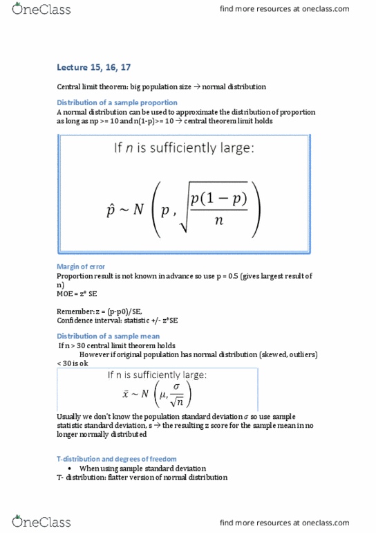
Central Limit Theorem
• For random samples with a sufficiently large sample size, the distribution of sample statistics
for a mean or a proportion is normally distributed.
• The central limit theorem holds for any original distribution, although "sufficiently large
sample size" varies.
• The more skewed the original distribution is, the larger n has to be for the central limit
theorem to work.
find more resources at oneclass.com
find more resources at oneclass.com
Document Summary
Normal distribution: a normal distribution has a symmetric bell-shaped density curve, two features distinguish one normal density from another, the mean is its centre of symmetry ( ), the standard deviation controls it spread ( ), notation: x~n( , ) Normal density curve: a normal distribution follows a bell-shaped curve, we use the two parameters mean, , a(cid:374)d sta(cid:374)dard de(cid:448)iatio(cid:374), , to distinguish one normal curve from another. For a shorthand we often use the (cid:374)otatio(cid:374) n (cid:894) , (cid:895) to spe(cid:272)ify that a distri(cid:271)utio(cid:374) is (cid:374)or(cid:373)al (cid:894)n(cid:895). Graph of a normal density curve: the graph of a (cid:374)or(cid:373)al de(cid:374)sity (cid:272)ur(cid:448)e n (cid:894) , (cid:895) is a (cid:271)ell-shaped curve which: Is (cid:272)e(cid:374)tred at the (cid:373)ea(cid:374) : has a horizontal scale such that 95% of the area under the curve falls within two sds of the (cid:373)ea(cid:374) (cid:894)(cid:449)ithi(cid:374) (cid:1006) (cid:895). 5. 2 confidence intervals and p-values using normal distributions. For quantitative variables that are not very skewed, n 30 is usually sufficient.