STAT 3006 Lecture Notes - Fall 2018 Lecture 6 - Homoscedasticity, Heteroscedasticity, Analysis of variance

Daniel T. Eisert STAT-3006
1
12.3 – Analysis of Variance (ANOVA) Assumptions
Chapter XII: Analysis of Variance
One-Way ANOVA
Model Conditions
Random sampling always produces chance variations. Any “factor effect” would
therefore show up in our data as the factor-driven differences plus chance
variations (“error”).
𝑫𝒂𝒕𝒂 = 𝑭𝑰𝑻 + 𝑹𝒆𝒔𝒊𝒅𝒖𝒂𝒍
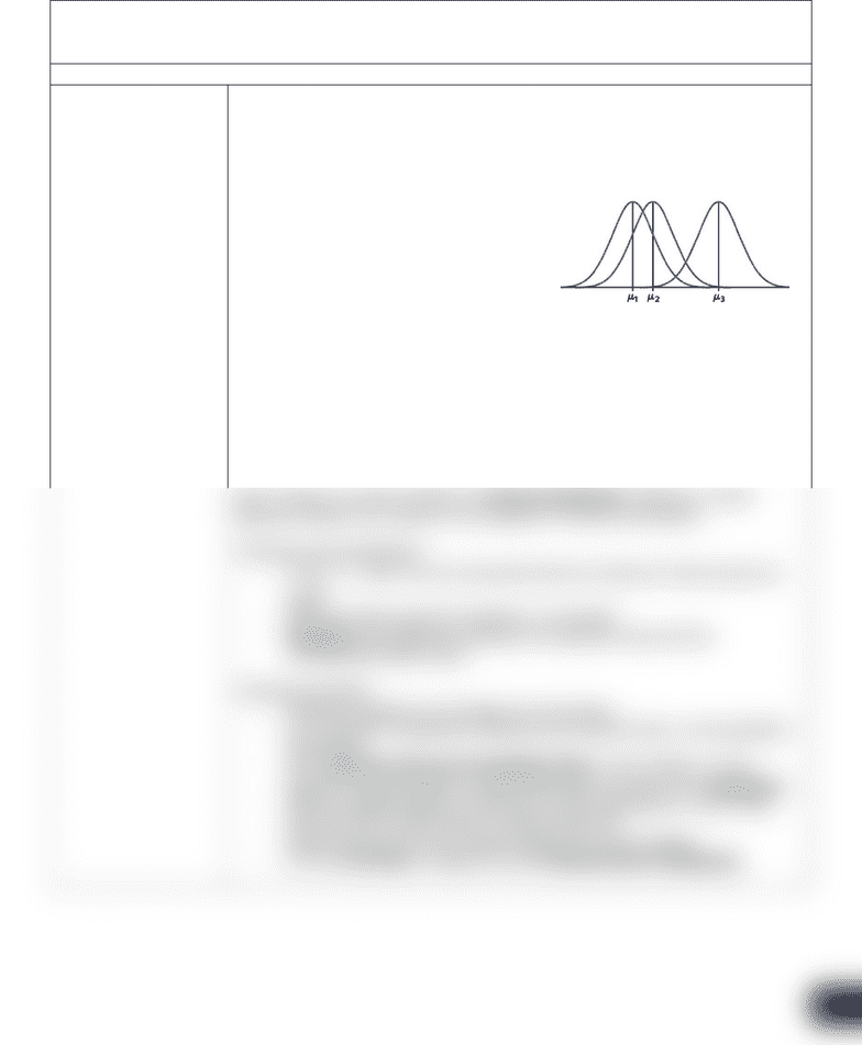
The one-way ANOVA model analyzes data 𝒙𝒊𝒋 where chance variations are
Normally distributed 𝑵(𝟎, 𝝈).
𝒙𝒊𝒋 = 𝝁𝒊+ 𝜺𝒊𝒋,
for 𝑰 = 𝟏, … , 𝑰 and 𝒋 = 𝟏, … , 𝒏𝒊. The 𝜺𝒊𝒋 are
assumed to be from a 𝑵(𝟎, 𝝈) distribution.
The parameters of the model are the
population means 𝝁𝟏,𝝁𝟐, … , 𝝁𝑰 and the
common standard deviation 𝝈.
Assumptions:
1. Data are collected using a SRS.
2. Independent samples.
3. Equal variance across all groups (homoscedasticity)
4. Population distribution for each group is approximately normal.
Homoscedasticity refers to moderate violations of equal population variances
not being serious. When the samples are equal (balanced) ANOVA works well
even if there is a severe problem of heteroscedasticity. Balance or nearly
balanced ANOVA’s are robust to the equality of variance assumption.
Checking Homoscedasticity:
- If 𝑠𝑚𝑎𝑥
𝑠𝑚𝑖𝑛 ≤ 2, then it can be assumed that the variances of each group are
equal.
- Check the data using the residuals vs. fits graph.
- Residual: the difference between the observed value and the
corresponding fitted value.
Checking Normality:
- Moderate violations of normality are not serious.
- It is a problem if graphical methods show extreme skew in the population
distribution.
- Use a QQ-Plot (Normal Probability Plot) to see whether or not a
dataset is approximately normally distributed; can also use a histogram.
- Data are plotted against a theoretical normal distribution in such a way
that the points should follow an approximate line.
- Departures from the line indicate departures from normality.
- In R, the PP-Plot is refered to as the Normal Plot of Residuals.
Document Summary
Any factor effect would therefore show up in our data as the factor-driven differences plus chance variations ( error ). (cid:2202)=+(cid:2187)(cid:2201)(cid:2191)(cid:2186)(cid:2203) The one-way anova model analyzes data (cid:2191)(cid:2192) where chance variations are. Normally distributed (cid:4666)(cid:2777),(cid:4667). (cid:2191)(cid:2192)=(cid:2191)+(cid:2191)(cid:2192), for =(cid:2778), , and (cid:2192)=(cid:2778), ,(cid:2191). The (cid:2191)(cid:2192) are assumed to be from a (cid:4666)(cid:2777),(cid:4667) distribution. population means (cid:2778),(cid:2779), , and the common standard deviation . Assumptions: data are collected using a srs, independent samples, equal variance across all groups (homoscedasticity, population distribution for each group is approximately normal. Homoscedasticity refers to moderate violations of equal population variances not being serious. When the samples are equal (balanced) anova works well even if there is a severe problem of heteroscedasticity. Balance or nearly balanced anova"s are robust to the equality of variance assumption. Checking homoscedasticity: (cid:3288)(cid:3289) 2, then it can be assumed that the variances of each group are. Check the data using the residuals vs. fits graph.

