STATS 10 Lecture Notes - Lecture 7: Binomial Distribution, Geometric Distribution, Standard Deviation

Chapter 6: Modeling Random Events: The Normal and Binomial Models
Probability distributions are models of random experiments
● Random: describes outcome of a scenario that canot be predicted w/ certainty
○ Event: outcome/set of outcomes from a random scenario
● Probability model: describes how we think data from a random scenario is generated→ represents a summary of
the unobservable data generating mechanism
○ We make an assumption that the probability model is a reasonably accurate description of how the data
is generated
○ We can tell if a model is good by how well the probabilities that the model predicts are matched by real-
life outcomes (just like the regression line)
● Distribution of a sample is a list that records
○ (1) the values that were observed in the data and
○ (2) the frequencies of these values
○ Distributions organize data to make comparisons and understand the variation in the data
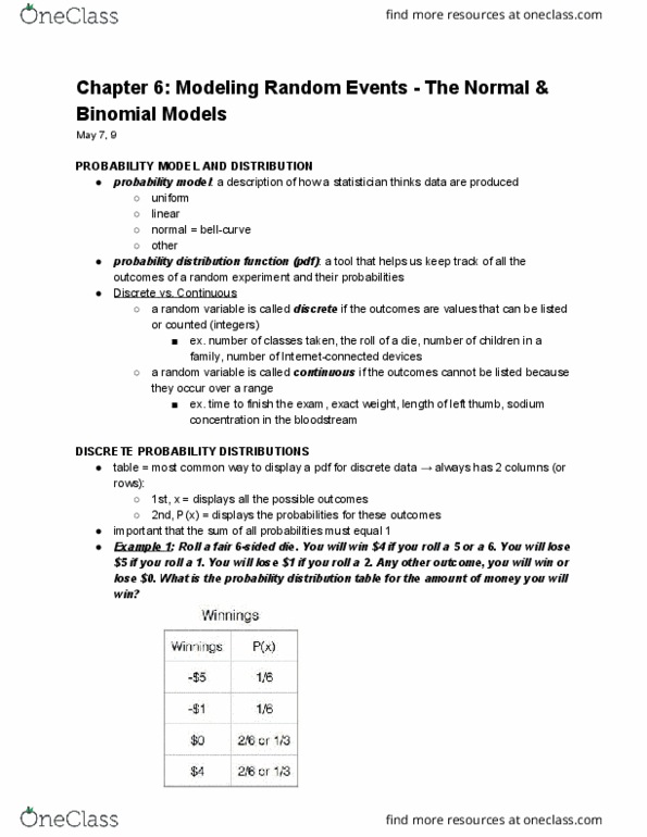
● Probability distribution/probability distribution function (pdf) = description of the random scenario that tells
us
○ (1) the possible outcomes of the random scenario
○ (2) the probability of each outcome
● OF NUMERICAL VALUES, we can split the category into two subsections
○ Discrete outcomes/variables: numerical values that can be listed/counted
○ Continuous outcomes/variables: numerical values that occur over a range and cannot be
listed/counted
● Like how the way we visiualize data distribution depended on type of variable (numerical/categorical), the way we
describe/visualize a probability distribution will depend on the types of outcomes that are possible from a random
scenario (discrete or continuous)
○ Discrete: table/graph, can even
make a formula/equation
■ To make a graph for
discrete probability
distribution, we draw a
vertical line above the #
line where each outcome
value occurs, its height
proportional to each
outcome’s probability
■ Geometric distribution:
models the number of
independent trials until a
success
● E.g. probability of rolling a die x times until we see a 6 is
○ P(rolling x times) = (᪥)x-1 x (᪤)
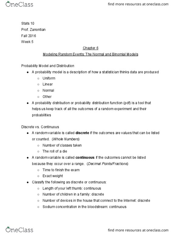
○ For continuous probability distributions, we cannot make a table to list
all possible outcomes since they occur over a RANGE of values →
focus on finding probability of a range of outcomes rather than
considering individual outcomes
■ Probability density curve → curve above x-axis where the
area under the curve for a given range (interval) of x-values
find more resources at oneclass.com
find more resources at oneclass.com
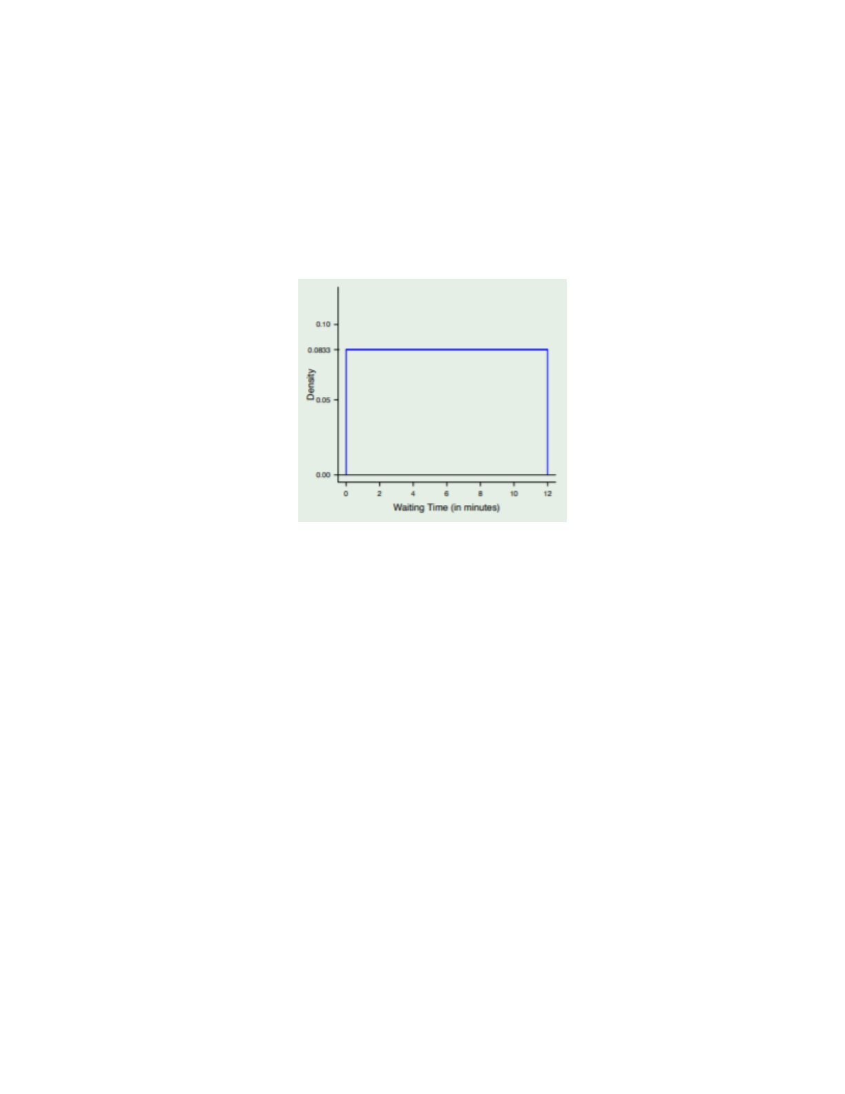
represents the probability that the outcome will be in that range
■ WARNING: the total area under the curve must be equal to 1! If not, the curve is not valid
● E.g. probability of wait time for coffee is 3-5 minutes
■ Probability density curve is usually a probability model → there is no way to observe enough
outcomes to have absolute certainty that the curve we use is the truth, so we make an
assumption that the probability model is a reasonable assumption of the underlying data
generating mechanism
● Many random phenomena have been shown to follow certain patterns that allow us to
have more confidence in certain settings
● continuous/uniform distribution: flat distribution shown below
○
The normal model
● Normal curve/distribution or bell curve/gaussian model: probability density curve that is symmetric and
unimodal
○ One of the most frequently used probability models in science
○ Features heaviliy in the Central Limit Theorem
○ Mean of a probability distribution= balancing point of a a probability distribution, denoted by mu (μ)
○ Standard deviation of a probability distribution = measures how far away the typical values are from
the mean, denoted by sigma (σ)
■ Do not confuse mean/standard dev of probability distributions w/ mean and standard deviations of
data (x¯ and s)
■ Mean and standard dev of probability distribution determines exact shape of normal distribution
● Normal distriution=perfect symmetric so mean=exact center
● wide/low normal curve has larger standard deviation (more area spread away from mean)
● narrow/tall normal curve has smaller standard deviation (more area clustered around
mean)
○ The notation N(μ, σ) represents a Normal distribution that is centered at the value μ (mean) and whose
spread is measured by the value σ (standard dev)
■ E.g. children’s heights, Normal model N(68, 2)
○ Since Normal distribution models continuous variables, area under the normal curve for a given range of
x-values represents the probability that the variable will be in that range
■ Probability of child will be taller than 65 inches is the same whether or not we include 65
inches → in continuous variables, strict inequality statements are interchangeable with non-strict
inequality statements
● This is NOT true for discrete variables
○ The formula for Normal curve and computing the area under the curve are both complicated! We use
either comp. Software or probability tables
find more resources at oneclass.com
find more resources at oneclass.com