STATS 10 Lecture Notes - Lecture 3: Standard Deviation, Missy Franklin, Box Plot


Chapter 3: Numerical Summaries of Center & Variation
April 9, 11, 16
INTRODUCTION
● in Chapter 2, we learned the features to always describe when considering a distribution
○ shape
- how many peaks, symmetric or skewed, any outliers
○ center
- the “typical” value
○ variability (spread)
- how spread out the data is
● In Chapter 3, we will learn about what values to use to measure center and spread
CENTER (the “typical value”)
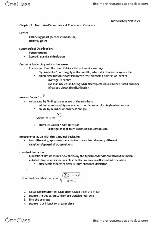
●mean
: the arithmetic average
= x=sum of all data values
number of data values n
∑x
●median
: the midpoint of ranked values
○ need to put the values in increasing order → the median will be the
value in the middle of the data set
○ if there is an even number of values, we take the average of the 2
middle numbers to find the median
●mode:
the most frequently observed value
SPREAD (how spread out the data is)
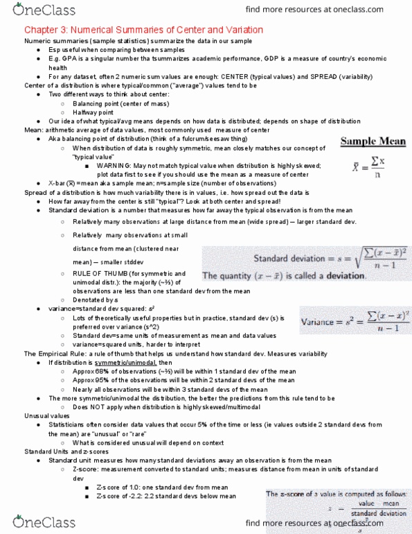
●standard deviation
: described by the square root of the variance (represents the typical
distance of a value from the mean)
σ =
√n − 1
∑ (x − x)²
○(x - x̄) means to take each data point, subtract the mean, and then square the
difference → called a deviation
○∑ (sigma) means to add up all the deviations
○n = the total number of data values
● Steps to Find the Standard Deviation:
1. Find the mean of your data
2. Subtract the mean from each data point, and then square those differences
3. Add (sum) all the squared values from Step 2
4. Divide the value from Step 3 by the number of your data points minus one → this
gives you the variance

5. Take the square root of Step 4 (the variance) to get the standard deviation
●Comparing Standard Deviations:
● interquartile range (IQR)
: the third quartile minus the first quartile
IQR = Q3 - Q1
○ Quartiles:
■ Q1 = first quartile (25% of the data are below this point)
● the median of the numbers less than Q2
■ Q2 = the median (50% of the data are below this point)
■ Q3 = third quartile (75% of the data are below this point)
● the median of the numbers greater than Q2
● range
: the maximum value minus the minimum value
range = max - min
○poor measure of spread, because:
■it is not resistant to outliers
■generally doesn’t tell us where most of the data is located
● measures of spread help us talk about what we don’t know
○ when the data values are tightly clustered around the center of distribution → the
IQR and standard deviation are small
○ when the data values are scattered far from the center → the IQR and standard
deviation are large
WHICH CENTER & SPREAD ARE BEST?
● when the distribution is symmetric and unimodal → use mean and standard deviation
● when the distribution is left- or right-skewed → use median and IQR
● when distribution is not unimodal → may be better to split the data:
○ in this case, neither the mean nor the median represent typical values or the
center
○ investigate further into possible separate sub-populations
○ present graphs & statistics of sub-populations separately
● Review:
○ shape
- how many peaks, symmetric or skewed, any outliers
○ center
- the “typical” value
■ use mean
for symmetric distribution
Document Summary
Chapter 3: numerical summaries of center & variation. In chapter 2, we learned the features to always describe when considering a distribution. In chapter 3, we will learn about what values to use to measure center and spread. Mean : the arithmetic average x = sum of all data values number of data values. Need to put the values in increasing order the median will be the value in the middle of the data set. If there is an even number of values, we take the average of the 2 middle numbers to find the median. Standard deviation : described by the square root of the variance (represents the typical distance of a value from the mean) N 1 gives you the variance. (x - x ) means to take each data point, subtract the mean, and then square the difference called a deviation. (sigma) means to add up all the deviations.