ECO 410 Lecture 14: 19

Get access


Related textbook solutions


Related Documents
Related Questions
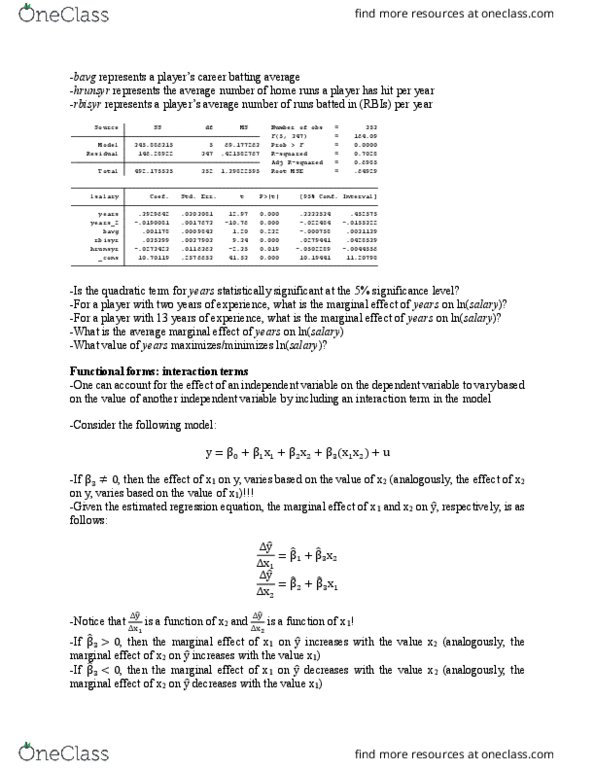
Suppose the following wage regression is run where the results are presented in a table below:
Wage = b0 + b1*Male + b2*Age + b3*Grade + b4*Married + b5*Experience
where the variables are as defined in class. Refer to the empirical results when answering the questions.
| Coefficients | Standard Error | t Stat | |
| Intercept | -7.856 | 0.404 | -19.444 |
| Male | 1.845 | 0.093 | 19.793 |
| Age | 0.123 | 0.015 | 7.902 |
| Grade | 0.677 | 0.021 | 31.920 |
| Married | 0.713 | 0.099 | 7.133 |
| Experience | 0.0096 | 0.0003 | 26.003 |
a) According to these regression results, do married individuals earn more than those non-married?
b) How much less would a female expect to earn on average than a male (when controlling for age, grade, marital status, and experience)?
c) Which variables are statistically significant at the 95 percent confidence level?
d) Calculate the average wage of a 20-year old married male with 16 years of education and 104 weeks of experience. Do the same for a 20-year old married female with 12 years of education and 0 work experience.
e) By how much will wages change with an additional year of education?
f) Suppose male are systematically more likely to be in a union than females and that union wages are higher than non-union wages. What effect will re-running this regression with a union dummy variable included have on the male coefficient?
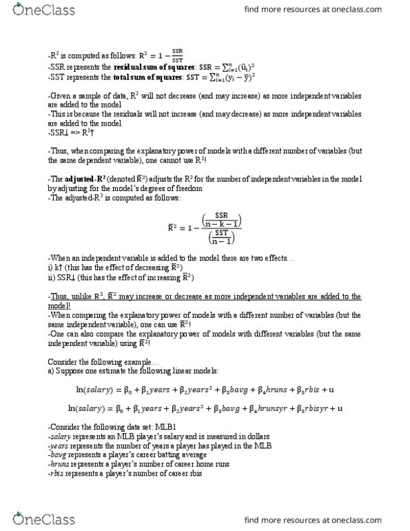
1. You are given only three quarterly seasonal indices and quarterly seasonally adjusted data for the entire year. What is the raw data value for Q4? Raw data is not adjusted for seasonality.
Quarter Seasonal Index Seasonally Adjusted Data
Q1 .80 295
Q2 .85 299
Q3 1.15 270
Q4 --- 271
2. One model of exponential smoothing will provide almost the same forecast as a liner trend method. What are linear trend intercept and slope counterparts for exponential smoothing?
A. Alpha and Delta
B. Delta and Gamma
C. Alpha and Gamma
D. Standard Deviation and Mean
3. When performing correlation analysis what is the null hypothesis? What measure in Minitab is used to test it and to be 95% confident in the significance of correlation coefficient.
A. Ho: r = .05 p < .5
B. Ho: r = 0 p >.05
C. Ho: r ? 0 p?.05
D. Ho: r = 0 p?.05
| In decomposition what does the cycle factor (CF) of .80 represent for a monthly forecast estimate of a Y variable? |
A. The estimated value is 80% of the average monthly seasonal estimate.
B. The estimate is .80 of the forecasted Y trend value.
C. The estimated value is .80 of the historical average CMA values.
D. The estimated value has 20% more variation than the average historical Y data values.
| 5. A Wendy's franchise owner notes that the sales per store has fallen below the stated national Wendy's outlet average of $1,368,000. He asserts a change has occurred that reduced the fast food eating habits of Americans. What is his hypothesis (H1) and what type of test for significance must be applied? |
A. H1: u ? $1,368,000 A one-tailed t-test to the left.
B. H1: u = $1,368,000 A two-tailed t-test.
C. H1: u < $1,368,000 A one-tailed t-test to the left.
D. H1: p < $1,368,000 A one-tailed test to the right
A. The rejection region and the t-table value generally gets smaller for sample size below 31. |
A. Yes. The data are significantly correlated through the 12th lag. C. No. Only the 12 lag period is not correlated. D. You cannot tell since the number of sample observations is not provided. E. The p-value is above .05 so the data is correlated. |
A. Type 2 error |
A. Yes. They move in the same direction as statistical significance. |
A. The weight cannot be calculated since the data observation is not given. |
A. Yes. The correlation coefficient is .873 that is greater than .05. |
A. Yes, since the residuals randomly vary in magnitude. |
A. -101.0 |
|