CAS MA 115 Lecture Notes - Lecture 6: Random Variable, Regional Policy Of The European Union, Simple Random Sample

1 May 2018
School
Department
Course
Professor

CHAPTER 6 – DISCRETE PROBABILITY DISTRIBUTIONS
Section 6.1 – Discrete Random Variables
Objective 1 – Distinguish Between Discrete and Continuous Random Variables
• Random Variable (X) – a numerical measure of the outcome from a probability
experiment
o Important to note this value is determined by chance
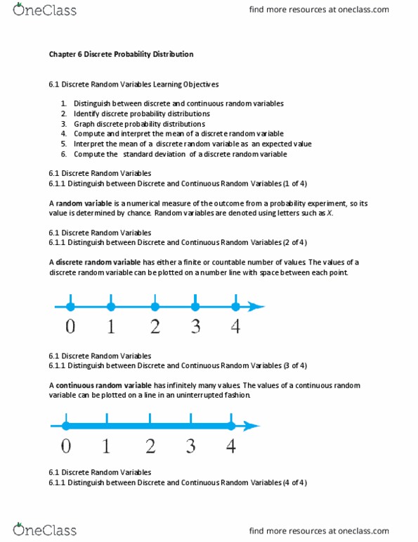
• Discrete Random Variable – has either a finite/countable number of values which can be
plotted on a number line with space in between
o Discrete; x = 0, 1, 2,…, 10
o Key Words: the number of, counting
o ex: the number of light bulbs that burn out in a room of 10 light bulbs in the next
year
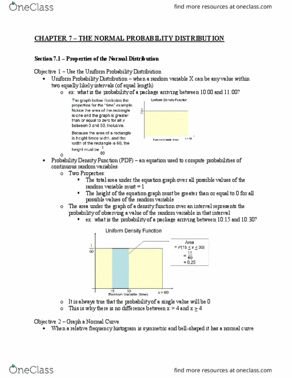
• Continuous Random Variable – has infinitely many values which can be plotted on a
number line in an uninterrupted fashion
o Continuous; t > 0
o Key Words: length, time, weight, height
o ex: the length of time between calls to 911
Objective 2 – Identify Discrete Probability Distributions
• Probability Distribution (of a random variable) – lists the possible values of the random
variable and their corresponding probabilities in the form of a table, graph or formula
• Rules:
o If P(x) denotes the probability that the random variable X = x, then
▪ 1. ΣP(x) = 1
▪ 2. 0 ≤ P(x) ≤ 1
Objective 3 – Graph Discrete Probability Distributions
• Can be graphed through a histograph
o Probability [P(x)] will be on the vertical axis
o Number of Individuals (x) will be on the horizontal axis
Objective 4 – Compute and Interpret the Mean of a Discrete Random Variable
• Formula = μx = Σ[xP(x)], where x is the value of the random variable and P(x) is the
probability of observing the value x
o Provides the likelihood of observing the value x
• ex: (0)(0.06) + (1)(0.58) + (2)(0.22) + (3)(0.10) + (4)(0.03) + (5)(0.01) = 1.49
o We would expect the mean number of DVDs rented to be 1 to 2
Objective 5 – Interpret the Mean of a Discrete Random Variable as an Expected Value
• As the number of repetitions of the experiment increases, the mean value of the n trials
will approach μX, the mean of the random variable X
• Essentially, as the number of trials of the experiment increases, the mean number of the
random variable X will be equal to mean of the probability distribution
find more resources at oneclass.com
find more resources at oneclass.com
Document Summary
Objective 3 graph discrete probability distributions: can be graphed through a histograph, probability [p(x)] will be on the vertical axis, number of individuals (x) will be on the horizontal axis. , x = [xp(x): ex: the data represents the number of dvds rented by 100 randomly selected customers in a single visit. Compute the mean number of dvds rented: as the number of trials of the experiment increases, the mean number of dvds rented approaches the mean of the probability distribution, which is 1. 49. The probability the female will survive the year is 0. 99791. Compute the expected value of this policy to the insurance company. 530 250,000 = -249,470: e(x) = (530)(0. 99791) + (-249,470)(0. 00209) = . 50, standard deviation formula. Objective 1 determine whether a probability experiment is a binomial experiment. Not rolling a 7), there is a set probability of success for each trial (p = 0. 5: ex2: n a class of 30 students, 55% are female.