MAT 1330 Lecture Notes - Lecture 3: T Helper Cell

• School: University of Ottawa
• Department: Mathematics
• Course: MAT 1330
• Professor: Rachelle Miron

Document Summary

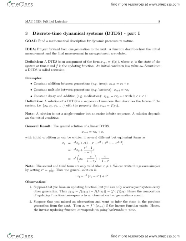
Goal: visualize the behavior of a dtds, identify special points. Graphing i: once we have calculated a solution, we can graph it as a sequence of points (0, x0), (1, x1), (2, x2),. (t, xt),. Graphing ii: without calculating a solution, we can visualize a solution of a dtds by using a technique called cobwebbing. Note: use the excel les available in the course material to generate your cobwebbing. The two plots below were generated using lineardtds. xls with updating function f(x) = The plot on the left shows the cobweb (updating function in red, diagonal in blue, cobweb in green), the plot on the right the solution as a function of time. De nition: a constant solution of a dtds is called a xed point or steady state or equilib- rium. A xed point is where the updating function intersects the diagonal. Xed point algebraically, one solves the equation x = f(x) for x.