BUSS1040 Lecture Notes - Lecture 2: Marginal Cost, Opportunity Cost, Market Power

28 May 2018
School
Department
Course
Professor

WEEK 2: PRODUCTION, COSTS AND SUPPLY
CHAPTER 7: PRODUCTION AND COSTS
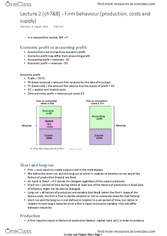
ECONOMIC PROFIT VERSUS ACCOUNTING PROFIT
• We assume firms aim to maximise profits
• Economic profit: revenues – total opportunity cost
o Total revenue (TR): amount a firm receives for sale of
its output
o Total cost (TC): amount a firm pays to buy inputs of
production + foregone opportunities
o Profit: total revenue – total costs
§
! " #$% &$'
§ Zero economic profit: revenues only cover
opp. costs
o E.g. B opens a restaurant, giving up a job as a lecturer that
pays $20 000 per year. He invests $50 000 of his savings in the restaurant and the current rate of interest is 10% p.a..
In year 1, the restaurant has revenue $200 000, rental costs $50 000 and food costs $20 000. What is B’s economic
profit in his Y1?
§ TR = $200 000
§ TC = explicit (rental $50 000 + food $20 000) + implicit (salary $20 000 + interest [$50 000 x 0.1]
= $95 000
§ Profit = $200 000 - $95 000
= $105 000
• Accounting profit: revenues – all explicit costs
THE SHORT RUN AND LONG RUN
• Short run: period of time during which at least one of the FOP is fixed
• Long run: all FOP are variable
• Defined in relation to how long it takes for all inputs to become variable à will differ b/w industries
PRODUCTION
• A firm converts inputs (labour, capital, land etc.) into final output (G+S) sold in the
marketplace
• Production function: shows relationship b/w quantity of inputs used and maximum
quantity of output produced, given the state of technology
• GRAPH: Marginal product (MP) - change in output when one more input is used
o Slope of production function
o Diminishing MP: MP becomes progressively smaller à each additional
worker contributes less to output than the worker before = capacity
§ Short run concept b/c relies on one input being fixed
• Long run production = all inputs are variable
o We are interested in how quantity of output changes when we change quantity of all FOP
§ Production function in LR:
( " )*+,-
o Returns to scale: how the quantity of an output changes when there is a proportional change in the
quantity of all inputs
§ Output increases by same proportional change = constant returns to scale
§ Output increases by more than proportional increase in all inputs = increasing returns to scale
§ Output increases by less than proportional increase in all inputs = decreasing returns to scale
• Note: it is possible that a firm has diminishing MP in short run, and has increasing returns to scale in long run
Document Summary
Economic profit versus accounting profit: we assume firms aim to maximise profits. Zero economic profit: revenues only cover opp. costs. B opens a restaurant, giving up a job as a lecturer that pays 000 per year. He invests 000 of his savings in the restaurant and the current rate of interest is 10% p. a In year 1, the restaurant has revenue 000, rental costs 000 and food costs 000. Tc = explicit (rental 000 + food 000) + implicit (salary 000 + interest [ 000 x 0. 1] = 000: accounting profit: revenues all explicit costs. Short run: period of time during which at least one of the fop is fixed. Long run: all fop are variable: defined in relation to how long it takes for all inputs to become variable will differ b/w industries. Short run concept b/c relies on one input being fixed.