BUSS1020 Lecture Notes - Lecture 6: E.G. Time, Standard Deviation, Exponential Distribution

13 Sep 2018
School
Department
Course
Professor

Week 6- Continuous Probability Distributions:
- Continuous rvs can assume any value on a continuum (uncountable number of
values)
- Continuous distributions have 3 forms:
o Normal distribution
o Uniform distribution
o Exponential distribution
- For any continuous rv X, P(X=a) is 0 because there is always going to be a fractional
variation (e.g. prob of being exactly 2m tall)
- Hence we consider prob within a range P(a<X<b)
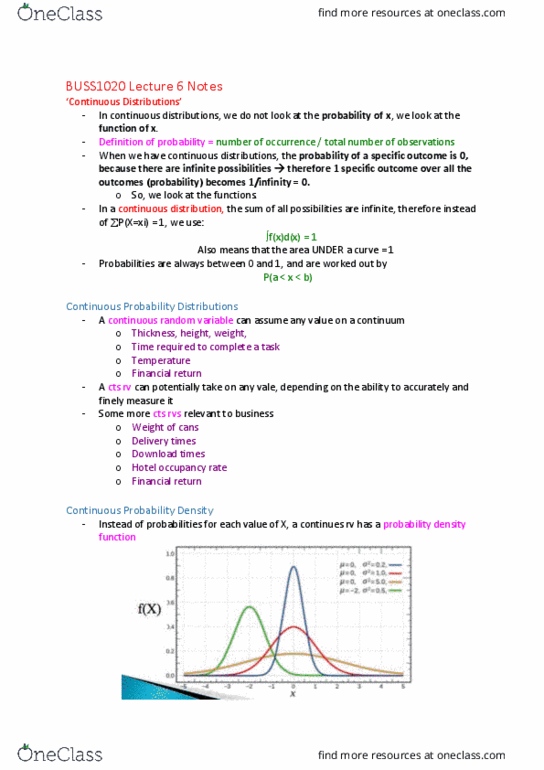
- This probability is the AREA under the ‘probability density function’ curve between
a and b
- The total area under the density curve between -∞ and +∞ is 1
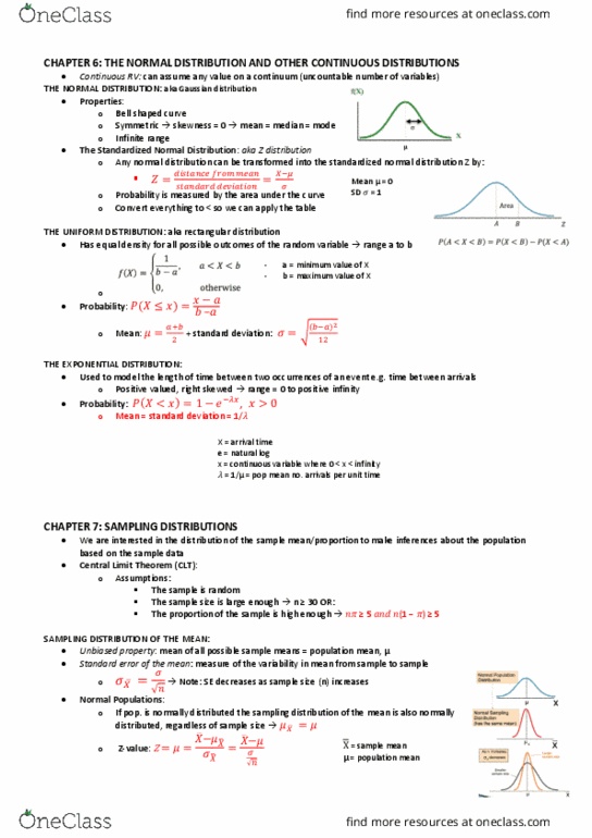
The Normal Distribution:
- Features:
o Bell-shaped
o Symmetric around the mean
o Mean, median and mode are equal (note that mode cannot be 1 fixed value in
continuous distribution; we look at a small interval and pick the mode
interval)
- Parameters:
o 𝜇= location given by the mean
o = standard deviation
- Has an infinite theoretical range +∞ to -∞; - meaning in theory could be this far from
mean, but usually within a few stdevs
- There is a family of normal distributions- infinite depending on the varying
parameters (mean/stdev)
The Standardised Normal:
- Any normal distribution can be transformed into the STANDARDISED normal
distribution (Z)
- We want this standardised normal distribution so that everyone uses same one
- It has 𝜇=0 and =1
- This is done by transforming X units (normal) into Z units (stand)
- To standardise a normal value:
o Find the Z-score:
Document Summary
Continuous rvs can assume any value on a continuum (uncountable number of values) Continuous distributions have 3 forms: normal distribution, uniform distribution, exponential distribution. For any continuous rv x, p(x=a) is 0 because there is always going to be a fractional variation (e. g. prob of being exactly 2m tall) Hence we consider prob within a range p(a