KIN 3982 Lecture Notes - Lecture 8: Pearson Product-Moment Correlation Coefficient, Null Hypothesis, Observational Error

55 views3 pages

sangriarat520

28 Feb 2019

School

Department

Course

Professor

For unlimited access to Class Notes, a Class+ subscription is required.

Document Summary

If the statistics reveal that there is a 95% chance that the null hypothesis is false, then p is said to be 0. 05. Chi square: analysis used when dependent variable is categorical. Determine if the distribution to groups is due to changes in the independent variable or random error. Overview of data analysis: tests of relationship (e. g. , regression, typically used for surveys, statistical tests of difference (e. g. , anvoa, t-test, typically used for experimental designs. Regression: bivariate regression: how well one variable predicts the value of a second variable (i. e. , dependent or criterion variable, multiple regression: how well multiple variables predict (i. e. , predictors) the value of another variable. T-test (two group designs: t-test: examines if two groups significantly differ from one another, what increases the likelihood of a significant t-test, larger sample size, larger differences between the means, low variability in the sample.

Related Questions

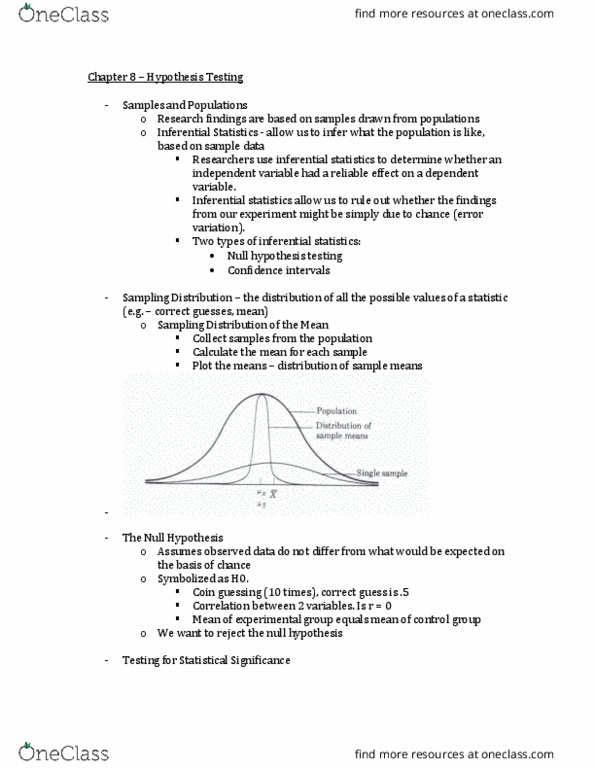
Introduction: A Chi-square test is used to compare observed data with expected data according to a hypothesis. For instance, if you were crossbreeding 2 heterozygous pea plants, you would expect to see a 3:1 phenotypic ratio in the offspring. In this case, if you were to breed 400 pea plants, you would expect to see 300 plants showing the dominant trait and 100 showing the recessive trait. But what happens if you observe only 260 plants with the dominant trait and 140 plants with the recessive trait? Does this mean something is wrong with Mendelian genetics or is this difference in expected results just due to chance (random sampling error)? These are the questions that can be answered using Chi-square statistics. The results of this statistical test is used to either reject or accept (fail to reject) the null hypothesis. The null hypothesis states there is no significant difference between the observed results and the expected results. This means that if the null hypothesis is accepted, the difference in observed and expected results was just a matter of chance and so the observed results basically "fit" with what was expected. Degrees of freedom (df) = number of independent outcomes (Y) being compared less 1 df = Y-1 At the 95% confidence interval we are 95% confident that there is a significant difference between the observed and expected results, therefore rejecting the null hypothesis. Probability Value - Is the decimal value determined from the X2 table and is the probability of accepting the null hypothesis. A 0.05 probability value equates to a 95% confidence interval.

The Chi-squared test formula is: Example: If we cross two pea plants that are heterozygous yellow pods, we would expect a 3:1 phenotypic ratio. So let's say we actually did the cross and got 280 plants with green pods and 120 plants with yellow pods. Question: Is this a 3:1 phenotypic ratio? This is the value of Chi-squared Test. We have a total of 400 plants and we expect a 300 green:100 yellow phenotypic ratio If the calculated Chi-squared value is less than the critical value listed in the Chi-squared table, then we accept the null hypothesis. This means that there is no significant difference between the observed and the expected values. Our degrees of freedom (df) = 2 outcomes - 1, or df = 1. Now we go the X2 table below and using the df = 1 and probability value of 0.05, our critical value is 3.84. Since our calculated X2 value is 5.33, and is larger than the critical value, we reject the null hypothesis and can say (at 95% confidence) that there is a significant difference between our observed and expected values.

The parent generation is yellowed podded and green podded pea plants. You cross a yellow podded pea plant with a green podded pea plant and you get 100% yellow podded plants in the F1 Generation (Phenotypic ratio 4 : 0, yellow to green). What will be the expected phenotypic ratio when you allow the F1 generation to reproduce?

Fill out the Punnett square.

If we actually did the cross and got 1150 yellow and 350 green. Would this be a consistent with what was expected?

Learning Outcomes Questions

1. Why would you run a Chi-squared test?

To determine if our data is consistent with expected results.
		a To determine if our data is consistent with expected results. b To determine if our data exactly matches the expected results.
		c To determine the expected results.
	d	To compare the phenotypic ratios to the genotypic ratios.

2. Determine the degrees of Freedom of the phenotypic ratio for this genetic cross.

a. 1

b. 2

c. 3

d. 4

e. 5

3. Using the data given, what is the result of your Chi-squared analysis? x2= ___.

	a.	2.22
	b	2.71
	c	4.36
	d	187.78
	e	448.27

4. Using the results of your Chi-squared analysis, do we fail to reject or reject the null hypothesis?

a.		Fail to reject the null
b.		Reject the null
c.		It cannot be determined from the data given

silversalmon27

ECON 3050

Q24. The coefficient of determination (r²) is calculated as 0.49, then the correlation coefficient:

Cannot be determined without the data

Should be - 0.70 or 0.70

Should be 0.

Neither of the above

Q25. A regression line is used for all of the following except one. Which one is not a valid use of a regression line?

To estimate the average value of Y at a specified value of X.

To predict the value of Y for an individual, given that individual's X-value.

To estimate the change in Y for a one-unit change in X.

To determine if a change in X causes a change in Y.

Q26. Which choice is not an appropriate description of YË in a regression equation?

Estimated response

Predicted response

Estimated average response

Observed response

Q27. Which of the following is the best way to determine whether or not there is a statistically significant linear relationship between two quantitative variables?

Compute a regression line from a sample and see if the sample slope is 0.

Compute the correlation coefficient and see if it is greater than 0.5 or less than â0.5.

Conduct a test of the null hypothesis that the population slope is 0.

Conduct a test of the null hypothesis that the population intercept is 0.

Q28. There is no relationship between variables unless the data points lie in a straight line.

True

False

Q29. The sample regression analysis

Is the same as the population regression line

Is used to estimate the population regression line

Shows the true relation between dependent and independent variables

None of the above.

Q30. In regression, a dependent variable is sometimes called a predictor variable.

True

False

Q31. In a linear regression equation of the form y = a + bx, the intercept shows

The amount that y changes when x changes by one unit

The amount that x changes when y changes by one unit

The value of y when x is zero

The value of x when y is zero.

Q32. In a linear regression equation of y = a + bx, the slope b shows

Y / b

X / b

Y / X

X / Y

yellowturtle964

1. You are given only three quarterly seasonal indices and quarterly seasonally adjusted data for the entire year. What is the raw data value for Q4? Raw data is not adjusted for seasonality.

Quarter Seasonal Index Seasonally Adjusted Data

Q1 .80 295

Q2 .85 299

Q3 1.15 270

Q4 --- 271

2. One model of exponential smoothing will provide almost the same forecast as a liner trend method. What are linear trend intercept and slope counterparts for exponential smoothing?

A. Alpha and Delta

B. Delta and Gamma

C. Alpha and Gamma

D. Standard Deviation and Mean

3. When performing correlation analysis what is the null hypothesis? What measure in Minitab is used to test it and to be 95% confident in the significance of correlation coefficient.

A. Ho: r = .05 p < .5

B. Ho: r = 0 p >.05

C. Ho: r ? 0 p?.05

D. Ho: r = 0 p?.05

In decomposition what does the cycle factor (CF) of .80 represent for a monthly forecast estimate of a Y variable?

A. The estimated value is 80% of the average monthly seasonal estimate.
B. The estimate is .80 of the forecasted Y trend value.
C. The estimated value is .80 of the historical average CMA values.
D. The estimated value has 20% more variation than the average historical Y data values.

5. A Wendy's franchise owner notes that the sales per store has fallen below the stated national Wendy's outlet average of $1,368,000. He asserts a change has occurred that reduced the fast food eating habits of Americans. What is his hypothesis (H1) and what type of test for significance must be applied?

A. H1: u ? $1,368,000 A one-tailed t-test to the left.
B. H1: u = $1,368,000 A two-tailed t-test.
C. H1: u < $1,368,000 A one-tailed t-test to the left.
D. H1: p < $1,368,000 A one-tailed test to the right

6. As the sample size from a population increases, for a given level of significance what happens to the null hypothesis rejection region and size of the t-table value?

A. The rejection region and the t-table value generally gets smaller for sample size below 31.
B. The rejection region gets larger and the t-table value generally gets smaller for sample sizes below 31.
C. The rejection region remains unchanged while the t-table value gets smaller for all sample sizes.
D. The zero mean hypothesis region gets larger and the t-table value gets larger as well for sample sizes below 31.

7. You obtained autocorrelation LBQ value of 18.58 for the 12^th lag from a data sample. Are the data significantly correlated at the lag examined or not? You want to be 95% confident in your answer.

A. Yes. The data are significantly correlated through the 12th lag.
B. No. The data are not significantly correlated through the 12^th lag.

C. No. Only the 12 lag period is not correlated.

D. You cannot tell since the number of sample observations is not provided.

E. The p-value is above .05 so the data is correlated.

8. Sometimes forecasters get lazy or forgetful and do not check the significance of XY data correlations and use the X variable to forecast Y. What is the result of this?

A. Type 2 error
B. Autocorrelation error
C. Type 3 error
D. Type 1 error

9. Do error measures indicate the statistical significance of forecast model variables?

A. Yes. They move in the same direction as statistical significance.
B. Yes. As error measures decrease the variable significance increases.
C. No They indicate only the magnitude of estimate error.
D. No. They indicate only the statistical significance of a forecast or fitted values.

10. In exponential smoothing what is the weight of the alpha coefficient for a time series data observation from the 3^rd previous period if the original alpha value is set at .8?

A. The weight cannot be calculated since the data observation is not given.
B. The weight is zero since the alpha value is set relatively high.
C. .548
D. .0064

11.Given the data series below for variables Y (Monthly Inventory Balance) and X (Monthly Sales) are they significantly correlated at the 95% confidence level and how can you tell?

Ending Inv. Bal. Y		Monthly Sales X
1544		5053
1913		5052
2028		7507
1178		2887
1554		3880
1910		4454
1208		3855
2467		8824
2101		5716

A. Yes. The correlation coefficient is .873 that is greater than .05.
B. Yes. The correlation p-value is .002 which is less than .05.
C. No. The correlation coefficient is above the p-value.
D.No. The correlation p-value is greater than the 95% confidence level.

12. You have forecast the sales for your company for the last 12 months and the forecast residuals are shown below. Are these residuals to be considered random?
Residuals

-24

-348

-892

-62

-378

-489

-342

490

578

198

A. Yes, since the residuals randomly vary in magnitude.
B. Yes since the residuals are positive and negative and vary in magnitude.
C. No, since the residuals are stationary and vary in magnitude.
D. No, since the residuals indicate positive slope.

13. Given the residuals in problem 12 above what is the RMSE for the forecast?

A. -101.0
B. 411.8
C. 169603
D. 220.1

14. Which form of exponential smoothing can result in a na

KIN 3982 Lecture Notes - Lecture 8: Pearson Product-Moment Correlation Coefficient, Null Hypothesis, Observational Error

Document Summary

Get access

Related Documents

COM CM 321 Lecture Notes - Lecture 10: Type I And Type Ii Errors, Null Hypothesis, Contingency Table

CRIM 320 Lecture Notes - Lecture 3: Joint Probability Distribution, Conduct Disorder, Type I And Type Ii Errors

PSYC 2360 Lecture Notes - Lecture 8: Statistical Inference, Null Hypothesis, Mean Absolute Difference

Related Questions