STA 2023 Lecture Notes - Lecture 18: Probability Distribution, Random Number Generation

Document Summary
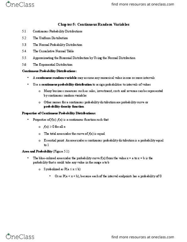
Ch 5 continuous random variables (skip 5. 4 and 5. 5) Continuous: can assume any value within some interval: ex. We will cover: uniform: equally likely outcomes, normal: bell shaped outcomes, exponential. Graphical form of a continuous random variable x is a smooth curve that might appear as shown: A = probability of what is going to happen between a and b. The curve is a function of x and is denoted by f(x). Called: probability density function or probability distribution: properties, total area under the curve is 1, p(x = a) = 0. If there is not shading, there is no probability. With discrete distribution, our probabilities massed at the possible values of x. With continuous distributions, our probabilities are found by looking for the area between two points. A continuous probability distribution where every value of x is equally likely over the range of values.