STAT 1450 Lecture Notes - Lecture 16: Central Limit Theorem, Confidence Interval, Statistical Inference

17 Sep 2020
School
Department
Course
Professor
Chapter 16, page 1
STAT 1450 COURSE NOTES – CHAPTERS 16
CONFIDENCE INTERVALS: THE BASICS
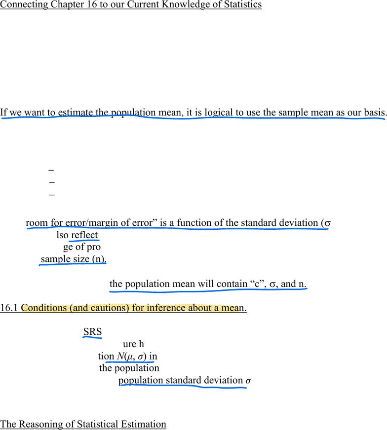
Connecting Chapter 16 to our Current Knowledge of Statistics
Midterm I material, Probability Theory,
Sampling Distributions (by way of the Law of Large Numbers, & the Central Limit Theorem)
have all laid the foundation for us to use sample statistics to estimate population parameters.
Statistical inference provides methods for drawing conclusions about a population from sample
data.
If we want to estimate the population mean, it is logical to use the sample mean as our basis.
But, the sample mean might not be exactly equal to the population mean.
S, e eed e f e.
Namely,
x
give or take “room for error”
x
“room for error”
x
“margin of error”
Thi f e/agi f e i a fci f he adad deiai (V).
But, it must also reflect
kedge f babii he (e a a ca c),
and the sample size (n).
The agi f e f he ai ea i cai c, V, and n.
16.1 Conditions (and cautions) for inference about a mean.
Here are three simple conditions (and cautions) for inference about a mean:
1. We have an SRS from the population of interest. The SRS may not be perfect.
2. The variable we measure has an exact An exact Normal distribution
Normal distribution N(μ, σ) in the population. is not always attainable.
3. We d k he ai ea μ. Sigh dd ha ed k σ,
But we do know the population standard deviation σ. but not μ.
The 3 ie cdii i fe be ai ee hgh hee i room for some doubt.
The Reasoning of Statistical Estimation
Even though we find the simple conditions a bit questionable, they help us understand the
reasoning of statistical estimation. Please read Example 16.1 on page 374 of the text, because it
goes through this reasoning well.
Chapter 16, page 2
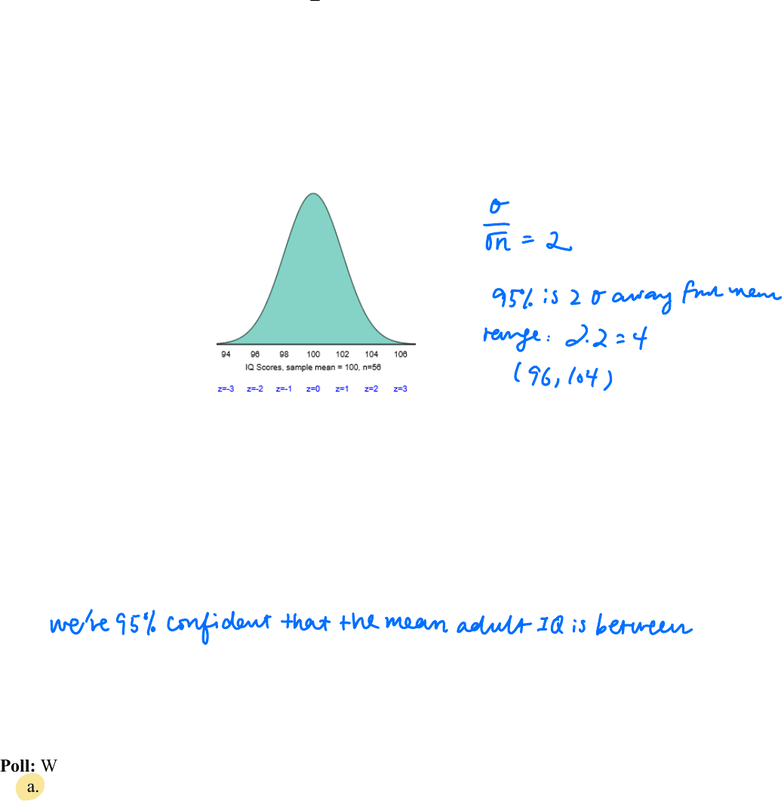
Example: Suppose IQ scores for adults follow a Normal distribution with a standard deviation of
15. A random sample of 56 adults yields an average score of 100. Recall that we do not know the
true mean IQ score.
1. To estimate the unknown population mean IQ score μ,
we can start with the mean
x
= 100 from the random sample.
2. Based on what we learned in Chapter 15,
we know the sampling distribution of the sample mean.
3. The 68-95-99.7 Rule and the sampling distribution for the sample mean ied
(--68%--)
(--- 95% ---)
(------ 99.7% --------)
4. If we focus uniquely on the 2nd interval, we would say:
Poll: What is the probability that the sample mean is exactly equal to the population mean?
a. 0
b. 0.5
c. 1
d. Sehig beee 0 ad 1, b e d k ha.
E
rn 2
95 is 20awayfmrmene
range 224
96 104
we're
95 confidentthat themean adult IQ isbetween
Document Summary
Connecting chapter 16 to our current knowledge of statistics. Sampling distributions (by way of the law of large numbers, & the central limit theorem) have all laid the foundation for us to use sample statistics to estimate population parameters. Statistical inference provides methods for drawing conclusions about a population from sample data. If we want to estimate the population mean, it is logical to use the sample mean as our basis. But, the sample mean might not be exactly equal to the population mean. S(cid:82), (cid:90)e(cid:182)(cid:79)(cid:79) (cid:81)eed (cid:86)(cid:82)(cid:80)e (cid:179)(cid:85)(cid:82)(cid:82)(cid:80) f(cid:82)(cid:85) e(cid:85)(cid:85)(cid:82)(cid:85). (cid:180) Namely, x give or take room for error . Thi(cid:86) (cid:179)(cid:85)(cid:82)(cid:82)(cid:80) f(cid:82)(cid:85) e(cid:85)(cid:85)(cid:82)(cid:85)/(cid:80)a(cid:85)gi(cid:81) (cid:82)f e(cid:85)(cid:85)(cid:82)(cid:85)(cid:180) i(cid:86) a f(cid:88)(cid:81)c(cid:87)i(cid:82)(cid:81) (cid:82)f (cid:87)he (cid:86)(cid:87)a(cid:81)da(cid:85)d de(cid:89)ia(cid:87)i(cid:82)(cid:81) ((cid:86)). But, it must also reflect (cid:82)(cid:88)(cid:85) k(cid:81)(cid:82)(cid:90)(cid:79)edge (cid:82)f (cid:83)(cid:85)(cid:82)babi(cid:79)i(cid:87)(cid:92) (cid:87)he(cid:82)(cid:85)(cid:92) ((cid:79)e(cid:87)(cid:182)(cid:86) (cid:86)a(cid:92) a c(cid:82)(cid:81)(cid:86)(cid:87)a(cid:81)(cid:87) c), and the sample size (n). The (cid:179)(cid:80)a(cid:85)gi(cid:81) (cid:82)f e(cid:85)(cid:85)(cid:82)(cid:85)(cid:180) f(cid:82)(cid:85) (cid:87)he (cid:83)(cid:82)(cid:83)(cid:88)(cid:79)a(cid:87)i(cid:82)(cid:81) (cid:80)ea(cid:81) (cid:90)i(cid:79)(cid:79) c(cid:82)(cid:81)(cid:87)ai(cid:81) (cid:179)c(cid:180), (cid:86), and n. 16. 1 conditions (and cautions) for inference about a mean.