FINS2624 Lecture Notes - Lecture 2: Risk Aversion, Risk Premium, Efficient Frontier


Lecture 4: Markowitz portfolio theory
- Dynamic optimisations in multiple periods
- Utility: used to assign values to every possible outcome- modelled depending only
on wealth- insatiation (greed) and risk aversion (fear)
- Risk aversion- prefer certainty to stochastic outcomes- risk premium (concavity)
- rf: compensates for generic inflation, market IR risk, liquidity risk
- Utility U(W) = ln(W), concavity ensures risk aversion
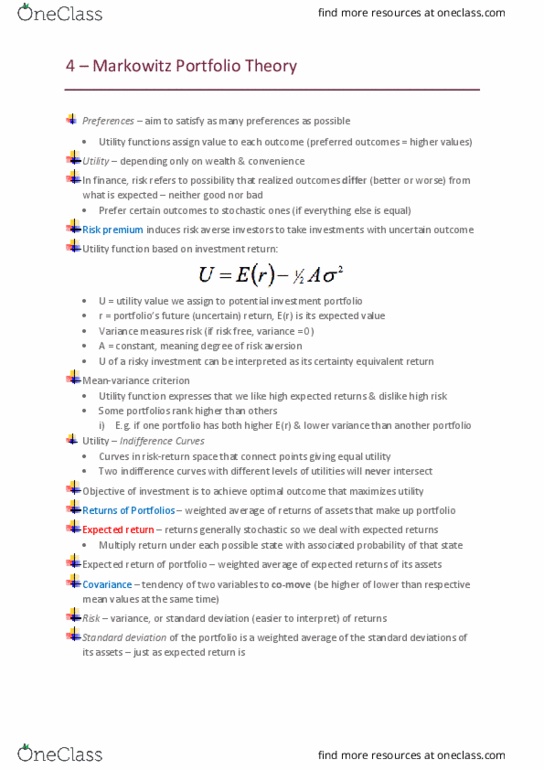
- Quadratic utility function: U = E(r) – ½ A *var(x) → U= certainty equivalent return
(A>0 for risk averse)
- rP= eighted ag of returs of portfolio= ∑ i*ri
a) Er= ∑ p*r
b) Expectations: Linear map conditions
c)
d)
e) covariance:
f)
▪
▪
▪
▪
▪
- (sum of var-cov
matrix)
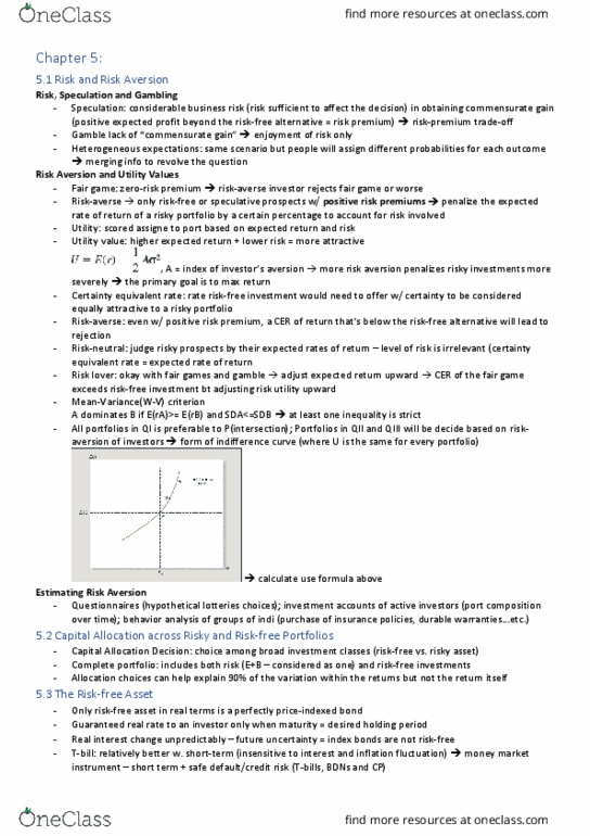
- Mean-variance criterion: high E(r) and lower s2
- Preferences: indifference curves (curves in risk-return space that connect points
giving = utility)
a) Indifference curves w different levels of utilities are parallel
→ up to n=3
- Diersifiatio: if p ≠ 1, portfolio sd ust e loer
find more resources at oneclass.com
find more resources at oneclass.com

- combination of 2+ more/less than perfectly correlated assets- risk reduction
diersifiatio eefit → combine many A w low correlations
a) if the A returns have low correlations, they are unlikely to realised below
their respective means at the same time – some risks cancel others out in
portfolio (-ve)
- pick on effiiet frotier fro p oards optiise utility ea-ariae
criterion
- optimal portfolio lies on tangent of indifference curve and investment frontier-
optimal portfolio
Lecture 5: Optimal Portfolios
- E(rf) = rf risk free return, var(rf)=0
- portfolio of risky and risk free A= complete porfolio
→ E(rc) = rf + y(E(rP) – rf)
where cov(rf,rp)=0 since Var(rf)=0
- expected return-vol of complete portfolio
find more resources at oneclass.com
find more resources at oneclass.com
Document Summary
Utility: used to assign values to every possible outcome- modelled depending only on wealth- insatiation (greed) and risk aversion (fear) rf: compensates for generic inflation, market ir risk, liquidity risk. Risk aversion- prefer certainty to stochastic outcomes- risk premium (concavity) Utility u(w) = ln(w), concavity ensures risk aversion. Mean-variance criterion: high e(r) and lower s2. Preferences: indifference curves (curves in risk-return space that connect points giving = utility: indifference curves w different levels of utilities are parallel. Pick on effi(cid:272)ie(cid:374)t fro(cid:374)tier fro(cid:373) (cid:373)(cid:448)p o(cid:374)(cid:449)ards (cid:894)opti(cid:373)ise utility(cid:895) (cid:858)(cid:373)ea(cid:374)-(cid:448)aria(cid:374)(cid:272)e(cid:859) criterion. Optimal portfolio lies on tangent of indifference curve and investment frontier- optimal portfolio. E(rf) = rf risk free return, var(rf)=0. Portfolio of risky and risk free a= complete porfolio. E(rc) = rf + y(e(rp) rf) where cov(rf,rp)=0 since var(rf)=0. We can form complete portfolios with any efficient risky portfolio- higher the slope of cal of an efficient risky portfolio, the better the risky portfolio is to form complete portfolios.